Surveying 6h5sx
This document was ed by and they confirmed that they have the permission to share it. If you are author or own the copyright of this book, please report to us by using this report form. Report r6l17
Overview 4q3b3c
& View Surveying as PDF for free.
More details 26j3b
- Words: 5,783
- Pages: 63
Purpose of Theodolite Traversing To provide control points for chain surveying, plane tabling and photogrammetric survey in flat country To fix the alignment of roads, canals, rivers, boundaries, etc. when better accuracy is required as compared to plane tabling To ascertain the coordinates of boundary pillars in numerical that can be preserved for future reference such as cantonment boundary pillars, forest boundary pillars, international boundary pillars, etc. In case the pillars get disturbed, their positions can be relaid with the help of their co-ordinates.
Principle of Theodolite Survey
Traverse Station • Station should be as minimum as possible. • Stable earth’s surface. Slope areas, muddy and too many plants should be avoided. • Stations can be seen clearly between each other.
Method of Measuring Traverse Angles Two types of traverse that are commonly used: • Traversing by interior angles • Traversing by bearings
• Traversing by Interior Angles To measure interior angle, traversing is carried out in one direction from one station to another station. They may be read either clockwise or counterclockwise as the survey progresses. It is good practice, however, to measure all angles clockwise. • Traversing by Bearings Topographic surveys are often run by bearings, a process that permits readings of all lines directly, thus eliminating the need to calculate them. Bearings are measured clockwise from the north end of the north point through the angle points. The theodolite is oriented at each set up by sighting to the previous station with back bearing on the circle.
Co-ordinates Normally, plane rectangular co-ordinates are used to identify the stations on a traverse. A specific point is defined by its perpendicular distances from each of two co-ordinate axes which are based on north-south and east-west directions. The former is the reference axis and it can be: a) True north; b) Magnetic north; c) National Grid north; and d) A chosen arbitrary direction, which could be one of the traverse lines if so wished. The intersection of the axis given the origin for the survey and usually it is to the south and west to ensure that all points have positive co-ordinates.
Easting/northing The co-ordinates given by the perpendicular distances from the two main are termed:
Fig. 3.2
eastings (distance from the north-south axis) northings (distance from the east-west axis)
as indicated in Fig.3.2 for the points X and Y. Relative positions are given by co-ordinates differences E E Y E X and
N N Y N X
Bearings The position of a point may also be referenced by stating length XY and bearing ø of line XY, and these are referred to as polar co-ordinates. The bearing ø is termed the whole circle bearing (WCB) of XY. It is measured clockwise from 0˚ to 360˚ at X between the north-south reference direction and the direction of Y from X. In Fig.3.3 the whole circle bearing of YZ is θ, and the whole circle bearing of ZY is (θ − 180˚). Similarly for YX in Fig.3.2 the bearing is (ø + 180˚) and, in general of line 1− 2 = bearing of line 2 − 1 ± 180˚, 1 and 2 being points within the system.
Fig. 3.3
3.1
Calculation of bearings
a) Briefly explain the following (i) True north (ii) Magnetic north (iii)Whole circle bearings (WCB) b) The included angles gives in Table 3.1 are recorded at stations forming a closed traverse survey around the perimeter of a field. Table 3.1 Station A B C D E F
Included angle 122˚ 42´ 20″ 87˚ 16´ 40″ 133˚ 08´ 20″ 125˚ 55´ 20″ 92˚ 47´ 40″ 158˚ 06´ 40″
Determine the amount of angular error in the survey and adjust the values of the included angles. If the whole circle bearing of the line BC is 45˚ calculate the whole circle bearings of the traverse lines and the corresponding values in the centesimal system. [Salford]
True north refers to the north geographical pole. The true or geographical meridian through a point is the trace of the plane through the north and south poles and the point in question. Magnetic north does not coincide with geographical north; the magnetic meridian is the direction revealed by a freely floating magnetic needle. The angle between it and the true meridian is termed declination. The whole circle bearing of a line has been defined previously as the angle, lying between 0˚ and 360˚, between the direction of north and the direction of the line, measured clockwise. Solution. Determine the angular error and apply corrections.
Figure 3.4
Figure 3.4 shows the traverse survey, the orientation of line BC being 45 from the meridian. This form of traverse is known as a closed-loop traverse since it begins and ends at the same point. The sum of the internal angles of a polygon is (2n − 4)*90 right angles, where n is the number of angles. Thus the sum of the six angles of this example must be eight right angles, or 720˚ 00´ 00″, whereas by measurement it is 719˚ 57´ 00″ (Table 3.2). The total error is therefore − 3´ 00″ or −180″, and hence a total correction of +180″ has to be applied. Note that this is of some magnitude and implies a relatively low order of work, for example fourth order implies an error of the 60 N sec, i.e. 60 6 147 " The corrections can be applied equally to each angle on the assumption that conditions were constant at the time of measurement and that the angle had been measured with the same accuracy. Hence a correction of (+180″/6) = +30″ is given to each angle in this example. Next we calculate whole circle bearings.
It is usual to proceed in an anti-clockwise manner round the traverse when internal angles have been measured. To determine the whole circle bearing of the line to the forward station it is necessary to add the whole circle bearing of the previous line, i.e. that from the back station, to the internal angle at the station, and then to add or deduct 180˚ depending upon whether that sum is less or greater than 180˚. For instance, at A we required the whole circle bearing of AF knowing that of BA. Table 3.2 Angle
Observed value
Correction
Adjusted value
A B C D E F
122˚ 42´ 20″ 87˚ 16´ 40″ 133˚ 08´ 20″ 125˚ 55´ 20″ 92˚ 47´ 40″ 158˚ 06´ 40″
+ 30″ + 30″ + 30″ + 30″ + 30″ + 30″
122˚ 42´ 50″ 87˚ 17´ 10″ 133˚ 08´ 50″ 125˚ 55´ 50″ 92˚ 48´ 10″ 158˚ 07´ 10″
Total
719˚ 57´ 00″
Total
720˚ 00´ 00″
Fig. 3.5
BA A 180 N B A BA S1 A B
Therefore from Fig. 3.5, WCB of AF Since
In this example we are given the bearing of BC but to move round the traverse in the anti-clockwise direction B, A, F, E, D, C, B we need the bearing of CB instead. Now whole circle bearing of BC = 45˚ Therefore whole circle bearing of CB = 45˚ + 180˚ = 225˚.
We can now proceed, using the quoted rule, to determine the whole circle bearing of the six traverse lines as follows.
Calculate centesimal values. In the centesimal system the major graduations of the instrument range from zero to 400 gon, as against zero to 360˚ in the sexagesimal system. Subdivision in the centesimal system is carried out in steps of ten and readings may be made to 0.0001 gon. It will be evident that: 1 degree is equivalent to 1 minute is equivalent to 1 second is equivalent to
10 gon 9 1 gon 54 1 gon 3240
Hence in the case of line FE, 53˚ 07´ 10″ in the centesimal system is equivalent 10 53 58.8889 to 9 1 7 0.1296 54 1 10 0.0031 3240 59.0216 gon
Similar calculations are used to complete table 3.3.
Table 3.3 Whole circle bearing Line
AF FE ED DC CB BA
Sexagesimal system
Centesimal system
75˚ 00´ 00″ 53˚ 07´ 10″ 325˚ 55´ 20″ 271˚ 51´ 10″ 225˚ 00´ 00″ 132˚ 17´ 10″
83.3333 gon 59.0216 gon 362.1358 gon 302.0586 gon 250.0000 gon 146.9846 gon
3.2 Correcting a traverse by Bowditch’s method A survey was carried out on a closed loop traverse with six sides. With the traverse labelled anti-clockwise as shown in Figure 3.6 the data in Table 3.4 were obtained. Table 3.4 Station
Internal angle
A B C D E F
130˚ 18´ 45″ 110˚ 18´ 23″ 99˚ 32´ 35″ 116˚ 18´ 2″ 119˚ 46´ 7″ 143˚ 46´ 20″
Length AB BC CD DE EF FA
14.248 85.771 77.318 28.222 53.099 65.914
Figure 3.6
The co-ordinates of point A are 1000 mE, 1000 mN and the whole circle bearing of the line A–F is 166˚ 45´ 52″. After adjustment by Bowditch’s method what are the co-ordinates of the other five traverse stations? [Salford/CIOB]
Solution. The first stage in the process is to determine the angular error and apply corrections as discussed in Example 3.1. Table 3.5 shows the tabulated angular data which sums to 720˚00´12″, expected closure 2n 4 90 720
error
720 00 '12 " 720 12 "
Thus, assuming that the angles have been measured with equal accuracy, a correction of – 2″ should be applied to each as shown in Table 3.5.
Table 3.5 Angle
Observed value
Correction
Adjusted value
A B C D E F
130˚ 18´ 45″ 110˚ 18´ 23″ 99˚ 32´ 35″ 116˚ 18´ 2″ 119˚ 46´ 7″ 143˚ 46´ 20″
–2″ –2″ –2″ –2″ –2″ –2″
130˚ 18´ 43″ 110˚ 18´ 21″ 99˚ 32´ 33″ 116˚ 18´ 0″ 119˚ 46´ 5″ 143˚ 46´ 18″
720˚00´12″
720˚00´00″
The next stage is to calculate the whole circle bearings. In Example 3.1 a method of calculating whole circle bearings was presented adding or subtracting 180˚ to the bearing of the back station plus the internal angle at the station. The same set of bearing can be obtained by approaching the problem differently. The reader is advised to try both methods and adopt the one that is found to be easiest; the two methods cannot be mixed in any one calculation.
Consider Fig. 3.7
Figure 3.7
WCB BA WCB AB 180 to lie in range 0 WCB BA 360
WCBBC WCBBA Bsubtract 360 if greater than 360
WCBCB WCBBC 180 etc
Readers can consider themselves to be at each of the stations in turn logically proceeding around the traverse in an anti-clockwise direction.
The next stage is to determine the easting and northing differences. In the introduction it was pointed out that: a) easting difference ΔE = EY – EX b) northing difference ΔN = NY – NX for points X and Y, which can be the stations at each end of a line as in Fig. 3.8. It will be seen that, ΔE = lXY sin (WCB) and ΔN = lXY cos (WCB).
Figure 3.8
The signs of ΔE and ΔN automatically follow the trigonometrical . Since the whole circle bearing lies between 180˚ and 270˚ both sin (WCB) and cos (WCB) are negative. This causes ΔN and ΔE to be negative in respect of the positive directions of N and E in Fig. 3.8.
The resultant easting differences and northing differences can now be computed for the traverse lines, as in Table 3.6. Table 3.6
Line
WCB
Length (m)
ΔE (m)
ΔN (m)
AB BC CD DE EF FA
297˚ 04´ 35″ 227˚ 22´ 56″ 146˚ 55´ 29″ 83˚ 13´ 29″ 22˚ 59´ 34″ 346˚ 45´ 52″
14.248 85.771 77.318 28.222 53.099 65.914
– 12.686 – 63.118 42.196 28.025 20.741 – 15.091
6.485 – 58.076 – 64.789 3.330 48.880 64.163
324.572
+ 0.067
– 0.007
Totals
Next, the closing error is determined. The algebraic sums of the easting differences and northing differences should be zero because the traverse starts and ends at A, but in fact we have total errors in so far as this traverse is concerned of ΔE = 0.067 m and ΔN = – 0.007 m Closing error = (ΔE2 + ΔN2) = (0.0672 + 0.0072) = 0.067 m Expressed fractionally in of the total length of the traverse the linear error is 0.067 m in 324.572 m or 1 in 4844. This is close to third-order accuracy of 1 in 5000.
The error in easting and northing distances should now be corrected. There are a number of methods of carrying out this task; Bowditch’s method is commonly adopted in civil engineering surveys since it has some theoretical background and relatively simple to apply. The method assumes that the error in the bearing of a line caused by inaccurate angular measurement produces a displacement at one end of a line (C) relative to the other end (B) which is equal and perpendicular to the displacement along that line due to an error in linear measurement, which is taken to the proportional to L BC . Figure 3.9 shows that the method causes C to be displace to C´, and consequently the bearing of BC changes.
Figure 3.9
For individual lines Bowditch’s method states:
correction to easting difference ΔEBC
dE lenght of line BC total lenght of traverse
correction to northing difference ΔNBC
dN lenght of line BC total lenght of traverse
in which dE and dN are total corrections required for the easting differences and northing differences, respectively. In this example dE = – 0.067 m and dN = + 0.07 m. Hence the corrections for line BC are: correction to easting difference 0.067
85.771 0.018m 324.572
correction to northing difference 0.007 85.771 0.002 m 324.572
Note also that in Fig. 3.9 the change in bearing of the line tan1
correction to E BC correction to N BC
dE dN This is the bearing of the closing error and the correction in bearing applies throughout the traverse for all lines. The corrections can be tabulated as in Table 3.7. Table 3.7 tan 1
Line
ΔE
Correcti on to ΔE
Corrected ΔE
ΔN
Correction to ΔN
Corrected ΔN
AB BC CD DE EF FA
– 12.686 – 63.118 42.196 28.025 20.741 – 15.091
– 0.003 – 0.018 – 0.016 – 0.006 – 0.011 – 0.013
– 12.689 – 63.136 42.180 28.019 20.730 – 15.104
6.485 – 58.076 – 64.789 3.330 48.880 64.163
+ 0.000 + 0.002 + 0.002 + 0.001 + 0.001 + 0.001
6.485 – 58.074 – 64.787 3.331 48.881 64.164
Totals
0.067
– 0.067
0.0
– 0.007
+ 0.007
0.0
The final stage is to determine the co-ordinates of the stations by applying the corrected difference ΔE and ΔN to the previous station co-ordinates, i.e. for B easting co-ordinates of B = easting co-ordinates of A + ΔEAB northing co-ordinates of B = northing co-ordinates of A + ΔNAB
Hence we obtain the values given in Table 3.8. Station
A (line AB) B (line BC) C (line CD) D (line DE) E (line EF) F (line FA) A
Co-ordinates E (m)
N (m)
1000.00 – 12.689 987.311 – 63.136 924.175 42.180 966.355 28.019 994.374 20.730 1015.104 – 15.104 1000.00
1000.00 6.485 1006.485 – 58.074 948.411 – 64.787 883.624 3.331 886.955 48.881 935.836 64.164 1000.00
Table 3.8
The following computer program will correct a closed-loop traverse by Bowditch’s method. Stations must be numbered clockwise around the traverse, the co-ordinates of point 1 being fixed and the whole circle bearing of the line ing station 1 and station N must be known. The internal angles at the stations should have been measured and the traverse lines must not cross. Line 230 in the program compares the actual angular misclosure to the allowable one and calculation stops if this is exceeded, this check can be removed by deleting lines 230 – 250. For readers with programmable calculators the DIM statement in line 20 has been set for a 10-sided traverse, minimum values are L(N). E(N+1), N(N+1), A(N), B(N). The data is output in a table and lines 430, 500, 540 and 560 will need to be reformatted for machines with a limited display.
3.3
Correcting a traverse by the Transit rule
A closed-loop traverse survey ABCDEA, shown in Fig. 3.10, gave the information in Table 3.9. Table 3.9 Line
Length (m)
Whole circle bearing
AB BC CD DE EA
293.27 720.83 497.12 523.34 761.87
45˚ 10´ 10″ 72˚ 04´ 55″ 161˚ 51´ 45″ 228˚ 43´ 10″ 300˚ 41´ 50″
Figure 3.10
Determine the closing error and hence, after adjustment by the Transit rule, determine the co-ordinates of the traverse stations given that the co-ordinates of A are 1200.00 mE, 1200.00 mN. It may be assumed that the whole circle bearings do not need an adjustment.
Introduction. The previous examples covered the first stage in traverse computation in that the measured angles were assessed for error, and then duly corrected. This was then followed by the determination of the whole circle bearings of the lines. This example allows us to follow the remainder of the procedure applied to the Transit rule. This method has to theoretical background, but it is such that if a line has no easting difference it will not be given an easting correction. This is not so with the Bowditch approach. The rule states
correction to ΔEDE correction to ΔNDE
dE E DE E
dN N DE N
Solution. First calculate the values of ΔE and ΔN in exactly the same manner to Example 3.2. The data are tabulated in Table 3.10. Table 3.10
Line
Length (m)
WCB
ΔE (m)
ΔN (m)
AB BC CD DE EA
293.27 720.83 497.12 523.34 761.87
45˚ 10´ 10″ 72˚ 04´ 55″ 161˚ 51´ 45″ 228˚ 43´ 10″ 300˚ 41´ 50″
+ 207.99 + 685.87 + 154.75 – 393.28 – 655.11
+ 206.76 + 221.77 – 472.42 – 345.27 + 388.94
Totals
+ 0.22
– 0.22
Sum
2097.00
1635.16
In the example ΔE = 2097.00 m and dE = – 0.22
also
ΔN= 1635.16 m and dN = + 0.22.
Magnitudes of the differences are considered but the signs are ignored. Thus for line DE we have correction to ΔEDE
0.22
393.28 0.04 2097.00
Table 3.11 Line
ΔE
Correction to ΔE
Corrected ΔE
ΔN
Correction to ΔN
Corrected ΔN
AB BC CD DE EA
+ 207.99 + 685.87 + 154.75 – 393.28 – 655.11
– 0.02 – 0.07 – 0.02 – 0.04 – 0.07
+ 207.97 + 685.80 + 154.73 – 393.32 – 655.18
+ 206.76 + 221.77 + 472.42 – 345.27 – 388.94
+ 0.03 + 0.03 + 0.06 + 0.05 + 0.05
+ 206.79 + 221.80 + 472.36 – 345.22 – 388.99
– 0.22
0.00
+ 0.22
0.00
correction to ΔNDE
345.27 1635.16 0.05 m. 0.22
For the complete traverse we obtain the values in Table 3.11.
To determine the co-ordinates of the stations we apply the corrected differences ΔE and ΔN to the previous station co-ordinates in the same manner as Example 3.2, and hence we obtain the values in Table 3.12.
Table 3.12 Station
A (line AB) B (line BC) C (line CD) D (line DE) E (line EA) A
Co-ordinates E (m)
N (m)
1200.00 207.97 1407.97 685.80 2093.77 154.73 2248.50 –393.32 1855.18 –655.18 1200.00
1200.00 206.79 1406.79 221.80 1628.59 –472.36 1156.23 –345.22 811.01 +388.99 1200.00
3.4 Vector misclosure of a traverse A five-dided loop traverse (whose angles have an accepted misclosure) has been computed giving the co-ordinate differences in Table 3.13 for each leg.
Table 3.13 Leg
ΔE (m)
ΔN (m)
AB BC CD DE EA
– 43.62 + 70.45 + 50.85 – 23.01 – 53.73
– 61.39 – 34.71 + 48.10 + 73.37 – 25.86
i. Determine the easting, northing and vector misclosure of the traverse. ii. The vector misclosure indicates a mistake of 1 m in the length of one of the sides of the traverse. Find which side contains the mistake and, after eliminating its effect, recomputed the easting, northing and vector misclosures. [London]
Table 3.14 Leg
E
N
AB BC CD DE EA
– 43.62 + 70.45 + 50.85 – 23.01 – 53.73
– 61.39 – 34.71 + 48.10 + 73.37 – 25.86
Misclosures
+ 0.94
– 0.49
Solution. (i) Calculate the vector misclosure of the traverse. The easting misclosure is + 0.94 m and the northing misclosure is –0.49 m, as indicated in Fig. 3.11. Whence vector misclosure
0.94
2
0.492
with a bearing oftan 1
1.06 m
0.94 117 32 ' , say. 0.49
Fig. 3.11
(ii) Now find the side that is in error. We are given that the angles as measured produced an acceptable micsclosure, and accordingly the magnitude of the misclosure cannot be attributed to their measurement. In such an eventuality we have to search for a side in the traverse which has the same bearing, approximately, as that of the closing error. Bearings have not been given in this example, but scrutiny of the data reveals that line BC is the only one whose easting difference and northing difference bear some proportional relationship with the corresponding difference of the closing error, i.e. +70.45 m for ΔE and – 34.71 m for ΔN against + 0.94 m and – 0.49 m, respectively, in the closing error. Thus we can assume that BC is in error by the amount stated. The apparent length of BC
70.45
2
34.71
78.54 m
Also, for BC,
E 70.45 2.03. N 34.71
E 0.94 1.92. N 0.49
2
If we accept that the length of BC should have been booked as 77.54 m (given that it has been subjected to an error of 1 m) and recalculate the magnitudes of the misclosures. Corrected ΔE for BC Corrected ΔN for BC
77.54 70.45 69.55 m 78.54 77.54 34.71 34.27 m 78.54
Thus for the amended closing error, ΔE = + 0.04 m Magnitude Bearing
0.04
tan 1
2
ΔN = – 0.05 m
0.05 0.06 m 2
0.04 141 19 '. 0.05
3.5 Closed-link traverse Measurements of the traverse ABCDE, as shown in Fig. 3.12, are given in Table 3.15. Table 3.15. Station
Clockwise angle
Length (m)
A B C D E
260˚ 31´18″ 123˚ 50´42″ 233˚ 00´06″ 158˚ 22´48″ 283˚ 00´18″
129.352 81.700 101.112 94.273
WCB of EY = 282˚ 03´00″
Figure 3.12
The measured angles are as shown in figure. Keeping the bearings XA and EY and also the co-ordinates of A and E fixed, obtain the adjusted co-ordinates for B, C and D using an equal shifts angular adjustment and Bowditch linear adjustment. [Bradford] Introduction. Although in an extended form, rather than starting and finishing at one point, this traverse is still a closed traverse, since it runs between two points whose co-ordinates are fixed and two lines whose bearings are fixed. It is known as a closed-link traverse can be readily adjusted.
Solution. Determined whole circle bearings. Starting with the bearing of XA we should end with the given bearing of EY; if not then there will be some angular error to balance.
This has to be shared out to five angles, i.e 21″ to A and E and 20″ to B, C and D. Next determine the easting and northing differences. Having adjusted the observed angles and deduced the whole circle bearings of the lines, the easting Table 3.16 Line
Length (m)
WCB
ΔE (m)
ΔN (m)
AB BC CD DE
129.352 81.700 101.112 94.273
203˚ 47´ 45″ 147˚ 38´ 47″ 200˚ 39´ 13″ 179˚ 02´ 21″
– 52.191 + 43.721 – 35.664 + 1.581
– 118.356 – 69.017 – 94.614 – 94.260
Total
406.437
– 42.553
– 376.247
Table 3.17 Point
E (m)
N (m)
E A
740.270 782.820
84.679 460.901
Differences
– 42.550
– 376.222
and northing differences are calculated for each line on the basic of E l sin WCB and N l cos WCB
From Table 3.16 it will be seen that the total difference is – 42.553 mE and – 376.247 mN. The fixed co-ordinates for A and E are as in Table 3.17. Thus the easting differences and northing differences given by the actual measurements are in error by eastings – 42.553 – (– 42.550) = – 0.003 m northings –376.247 – (– 376.222) = – 0.025 m
Therefore corrections of +0.003 m and +0.025 m are required for easting differences and northing distances, respectively. Make the Bowditch adjustment of the easting and northing differences. As stated previously the Bowditch linear adjustment for a particular line is correction to easting difference
lenght of line dE total lenght of traverse
correction to northing difference
lenght of line dN total lenght of traverse
in which dE = +0.003 m and dN = +0.025 m for this traverse. Hence the corrections to be applied are as in Table 3.18 and 3.19. The computation of co-ordinates is given in Table 3.20.
Table 3.18 Length (m) ΔE correction (m) ΔE correction (m)
AB
BC
CD
DE
Totals
129.352 + 0.001 + 0.008
81.700 + 0.000 + 0.005
101.112 + 0.001 + 0.006
94.273 + 0.001 + 0.006
406.437 + 0.003 + 0.025
Table 3.19 Line
Correction to
AB BC CD DE
+ 0.001 0.000 + 0.001 + 0.001
ΔE
Corrected ΔE – 52.190 + 43.721 – 35.663 + 1.582
– 42.550 m
Correction to + 0.008 + 0.005 + 0.006 + 0.006
ΔN
Corrected
ΔE
– 118.348 – 69.012 – 94.608 – 94.254
– 376.222 (Check)
Table 3.20 station
E (m)
Co-ordinates A ΔEAB
782.820 – 52.190
Co-ordinates B ΔEBC
730.630 – 43.721
Co-ordinates C ΔECD
774.351 – 35.663
Co-ordinates D ΔEDE
738.688 – 1.582
Co-ordinates E
740.270
N (m) ΔNAB
460.901 – 118.348
ΔNBC
342.553 – 69.012
ΔNCD
273.541 – 94.608
ΔNDE
178.933 – 94.254 84.679 (Check)
3.6 Errors introduced when centring the theodolite The magnitude of the errors in centring a theodolite over a station by various methods has been investigated and the following results quoted i.Plumb bob ± 3 mm ii.Centring rod ± 2 mm iii.Optical plummet ± 1 mm iv.Constrained centering ± 0.1 mm Compute the maximum errors in the measurement of a horizontal traverse angle of approximately 120 resulting from each of the above centering errors, assuming that the lengths of the adjacent drafts are 15 m and 25 m. [Eng. Council]
Figure 3.13
Introduction. In fig. 3.13 let the true centering position of the theodolite be S. It is possible for the vertical axis of the theodolite to lie anywhere within a circle of radius x from that point, x being one of the centering errors quoted above. However, there will be two points on the perimeter of that circle at which the true horizontal angle RST will be subtended. These are S1 and S2 which lie on the circumference of the circle containing R, S, and T. Accord-ingly
R S1 T R S T R S2 T because all three angles stand on chord RT.
Figure 3.14
Solution. First determine the maximum angular error due to a centring error of ±3 mm. In Fig.3.14 the theodolite has been centred at U, distance x from S. The measured horizontal angle
R U T 1 ,
Whilst the correct angle
R ST
Now
1
Therefore the error in measurement E sin sin But x z In which z TU
And In which
sin sin x y y UR
For small angles sin " sin 1 "
And Therefore
sin " sin 1 " E sec ond of arc x sin x sin y sin 1 " z sin 1 "
x sin sin sin 1 " y z It will be noted that absolute maximum error E is given when sin α and sin have their maximum values. This occurs when = 90˚ and θ = (γ − α) = 90˚, i.e. R S T 180 Note also that E increases as y and z decrease. However, in this case we are given that γ is of order of 120˚, and for the maximum error arising in this case dE 0 d
Now
E
Therefore Therefore Or
x sin sin sin 1 " y z x sin cos cos sin sin sin 1 " y z
dE x sin sin cos sin sin . d sin 1 " y z cos sin sin cos cos z y
y zsin tan cos
y z cos z sin 15 25 cos120 15 12.5 25 sin 120 21.65 1.2702078.
tan
Therefore
51 47 ' , say
The direction of displacement of U is significant. Taking case (i), x = 3 mm = 0.003 , thus
sin 51 47 ' 0.003 sin 120 51 47 ' E sin 1 " 15 25
0.003 0.92859 0.87568 sin 1 " 15 25
1 206265 sin 1 " and so E = 57.8 seconds.
In which
3.7 Errors due to maladjustment of the theodolite Derive expressions for the error in horizontal circle readings taken using a theodolite having the following maladjustments: i. The line of collimation not perpendicular to the trunnion axis by a small amount c. ii. The trunnion axis not perpendicular to the vertical axis by a small amount i. Hence prove that the effect of these of these maladjustments is eliminated by using the mean of face left and face right readings. Calculate the true value of angle PRQ from the reading given in Table 3.21 which were taken using a theodolite at R on face left only for which instrument c is known to be 23 seconds left and I is known to be 15 seconds down at the right
Table 3.21 Station
Horizontal circle
Vertical circle
P Q
27˚ 15′ 27″ 112˚ 27′ 53″
42˚ 15′ 12″ 28˚ 12′ 34″
Fig. 3.15
depression elevation
Introduction. In Fig. 3.15 the line of sight is shown to make a small angle c with the perpendicular to the trunnion axis (which would be its correct position). It sweeps along circle Z1QT1 when the telescope is rotated about the trunnion axis for the pointing on Q. The reading of the horizontal circle, however, is as if Q were in vertical circle ZS1 (to which Z1QT1 is parallel) whereas it is actually in vertical circle ZQ1. Consequently, the error in the horizontal circle reading is S1Q1 for this sighting, and it is positive on a clockwise reading circle.
Let SQ be at right angles to ZS1, i.e. S = 90˚. Then in spherical triangle ZSQ. sin Z sin S sin SQ
sin ZQ
sin SQ sin S sin ZQ For small angle we can write
Therefore
sin Z
SQ sin S z sin 90 1
Therefore
In which h QQ1 the altitude of Q SQ sin ce sin S 1 Z cos h SQ sec h
c sec h,
writing SQ c. In Fig.3.16 the left-hand of the trunnion axis is higher than the righthand and consequently the line of sight sweeps out Z2QS3, making angle i with the vertical ZS3. Q appears to be on that circle but is in fact on vertical circle ZQ2. Thus the error in horizontal circle reading for this particular case is S3Q2 and it is negative. Consider spherical triangle QQ2S3 in which Q2 = 90˚
sin Q 2S3 tan i tan QQ 2
Fig. 3.16 Therefore for small angles Q 2 S3 i tan h, in which h is the altitude of Q
The same expressions hold when depression angles are observed. In the case of collimation error c the senses of the errors are the same since path Z1QT1 is parallel to ZS1 throughout (see Fig. 3.15). However, in Fig. 3.16 Z2QS3 is inclined to ZS3, the two effectively crossing at S3 when moving from elevation to depression. Thus there is a change in sense and P, in this particular worker example, will have a positive error. When face right observations are made the paths of the lines of sight change direction Z1, moving to Z1′ in Fig. 3.15, thus giving an error of Q1S1 in the horizontal circle reading. This is of similar magnitude but of opposite sense to S1Q1. Similarly, in Fig. 3.16, Z2 moves to Z2′ and S3 to S4, giving error S4Q2 which is equal in magnitude but of opposite sense to error S4Q2 which is equal in magnitude but of opposite sense to error Q2S3. Thus in each case the means of the face left and face right observations will give the true value of the horizontal circle reading.
Solution. Determine angle P R Q. Tabulating the errors we have the values in Table 3.22. Table 3.22 Sighting
c sec h
i tan h
RP RQ
+ 23″ sec 42˚ 15′ 12″ = + 31.1″ + 23″ sec 28˚ 12′ 34″ = + 26.1″
+ 15″ tan 42˚ 15′ 12″ = + 13.6″ − 15″ tan 28˚ 12′ 34″ = − 8.0″
Applying corrections equal and opposite in sense to the above errors we obtain the values given in Table 3.23.
Table 3.23 Sighting
Observed angle
Net correction
Corrected angle
RQ RP
112˚ 27′ 53″ 27˚ 15′ 27″
− 18.1″ − 44.7″
112˚ 27′ 34.9″ 27˚ 14′ 42.3″ 85˚ 12′ 52.6″
Therefore the corrected angle P R Q 85 12 ' 53 " to the nearest second.
Related Documents 171j1w

Surveying 6h5sx
November 2022 0
Surveying 6h5sx
December 2020 0
Surveying 6h5sx
November 2019 86
Surveying 6h5sx
November 2021 0
Surveying 6h5sx
April 2020 47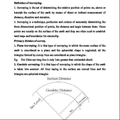
Chain Surveying And Com Surveying 1r582t
November 2021 0More Documents from "Shazrin Yusof" p581k
Surveying 6h5sx
November 2021 0
Pds - Sika Monotop-412 My (1) 574za
December 2021 0
All About Ost Sassy Girl 6z3i64
September 2022 0
Cara Menulis Khat Nasakh Step By Stepxx 172v3h
December 2019 163
Elevator System Using Microcontroller 316c3r
November 2019 80