Strata 3y5to
This document was ed by and they confirmed that they have the permission to share it. If you are author or own the copyright of this book, please report to us by using this report form. Report r6l17
Overview 4q3b3c
& View Strata as PDF for free.
More details 26j3b
- Words: 15,859
- Pages: 309
STRATA: Seismic Inversion Workshop
STRATA Course Outline Overview of Post-stack Inversion Exercise 1 - Erskine 3D – Initializing Model Building 1: Log Correlation Exercise 2 - Erskine 3D - Log Correlation and inversion Model Building 2: terpolation Wavelet Extraction Exercise 3 - Blackfoot - Starting the Project Model-based Inversion Parameters Exercise 4 - Blackfoot – Model-based Inversion Other Inversion Parameters Exercise 5 - Blackfoot – Other Inversion Methods Appendix: Overview of Pre-stack Inversion Exercise 6 – Simultaneous inversion of pre-stack data February, 2011
2
General Inversion Comments
Inversion is the process of extracting, from seismic data, the underlying geology which gave rise to that seismic. Traditionally, inversion has been applied to post-stack seismic data, with the aim of extracting acoustic impedance volumes (Strata). Recently, inversion has been extended to pre-stack seismic data, with the aim of extracting both acoustic and shear impedance volumes. This allows the calculation of pore fluids (Strata + AVO). Another recent development is to use inversion results to directly predict lithologic parameters such as porosity and water saturation (Emerge).
February, 2011
3
General Inversion Comments Input Seismic Post-stack seismic inversion transforms an input seismic volume into a volume of acoustic impedance.
Acoustic Impedance This output display shows 3 components: (1) (2) (3)
Derived AI (colour) Derived AI (wiggle) Real AI logs
February, 2011
4
Types of Inversion These inversion methods are available in STRATA: Post-stack: Recursive: Model Based: Sparse Spike: Colored:
Traditional bandlimited inversion Iteratively updates a layered initial model Constrained to produce few events Modern derivative of Recursive Inversion
Pre-stack:
February, 2011
Elastic Impedance:
Enhancement for pre-stack data
Independent Inversion: Lambda-mu-rho (LMR):
Enhancement for pre-stack data Enhancement for pre-stack data
Simultaneous Inversion:
Enhancement for pre-stack data 5
General Forward Model for Inversion The common forward model for all inversions:
Wavelet
Impedance
Reflectivity
Seismic
Acoustic Shear Elastic February, 2011
6
Inverse Model Inversion tries to reverse the forward model:
Inverse Wavelet
Seismic
Reflectivity
Impedance Acoustic Shear Elastic
February, 2011
7
General Forward Model for Inversion Impedance
Reflectivity
Z i 1 Z i Ri Z i 1 Z i
Z=
Acoustic Impedance =
Acoustic Impedance or Shear Impedance or Elastic Impedance
Ri
Zi+1
VP VS
Shear Impedance
=
Elastic Impedance
= Complicated formula (later)
February, 2011
Zi
8
General Forward Model for Inversion Reflectivity
Seismic
S W * R Noise
Seismic = Wavelet convolved with Reflectivity plus noise.
Notes (1) (2) (3) (4)
February, 2011
There are no multiples modeled. Transmission loss and geometric spreading are ignored. Frequency-dependent absorption is ignored. The wavelet may be time varying.
9
General Forward Model for Inversion
The effect of convolving the wavelet with the reflectivity is to remove much of the highfrequency detail:
February, 2011
10
General Forward Model for Inversion
Convolution in the time domain is multiplication in the frequency domain. As we can see from these plots, the effect of the wavelet is to remove both high and low frequencies from the trace spectrum. Theoretically, inversion attempts to recover these lost regions.
February, 2011
11
Non-Uniqueness in Inversion All inversion algorithms suffer from “non-uniqueness”. There is more than one possible geological model consistent with the seismic data. The only way to decide between the possibilities is to use other information, not present in the seismic data. This other information is usually provided in two ways: • the initial guess model • constraints on how far the final result may deviate from the initial guess The final result always depends on the “other information” as well as the seismic data. February, 2011
12
Non-Uniqueness in Inversion Initial Model
Seismic
+
Inversion
February, 2011
13
Bandlimited (Recursive) Inversion Recursive Inversion, also called Bandlimited Inversion, is the simplest and earliest form of inversion. Starting from the definition of reflection coefficient:
The impedance of the ith + 1 layer can be determined from the ith layer: Starting at the first layer, the impedance of each successive layer is determined by recursively applying this formula: February, 2011
Z i 1 Z i Ri Z i 1 Z i 1 Ri Z i 1 Z i 1 Ri n 1
Z n Z1
i 1
Zi Ri Zi+1
1 Ri 1 Ri 14
Bandlimited Inversion Z (m/s*g/cc)
In this simple example: (a) shows that we can recover the true value of impedance if we have a single spike, but (b) shows that if we convolve the spike with a wavelet we cannot recover the correct value of impedance.
Z1 = 1000
Z2 = 1500
Z1 = 1000 Z2 = 818 Z3 = 1227 Z4 = 1004
February, 2011
15
Bandlimited Inversion Step 1: The initial background model for Recursive Inversion is formed by filtering an impedance log from a well:
10-Hz High Cut
February, 2011
16
Bandlimited Inversion Step 2: The recursive equation is applied to the seismic trace. (Note: this is almost identical to a -90 degree phase rotation):
1 ri Zi 1 Zi * 1- ri
February, 2011
17
Bandlimited Inversion Step 3: Add the scaled inversion trace to the filtered model to get the final result:
+
February, 2011
=
18
Bandlimited Inversion Input Seismic Recursive Inversion produces a result which is bandlimited to the same frequency range as the input seismic data. Note the loss of high frequency detail, as compared with the well logs.
February, 2011
Recursive Inversion
19
Bandlimited (Recursive) Inversion
Issues in Recursive Inversion: (1) The wavelet is ignored. This means that the input seismic data must be zero phase. STRATA automatically “dephases” the data if an extracted wavelet is available.
(2) Even if the seismic is zero-phase, side-lobes from the actual wavelet will be interpreted by the algorithm as lithologic variations. (3) The inversion result is bandlimited to the frequency range of the seismic data. (4) The scaling of the seismic trace to reflectivity is critical to get the proper range of impedance changes.
February, 2011
20
Model Based Inversion Model Based Inversion starts with the equation for the convolutional model:
S W * R Noise Assume that the seismic trace, S, and the wavelet, W, are known. Assume that the Noise is random and uncorrelated with the signal. Solve for the reflectivity, R, which satisfies this equation. This is actually a non-linear problem, so the solution is done iteratively.
February, 2011
21
Model Based Inversion Step 1: The initial background model for Model Based Inversion is formed by blocking an impedance log from a well:
The specifies the layer size in milliseconds. All the layers are originally set to the same size (in time).
February, 2011
22
Model Based Inversion Step 2: Using the blocked model, and the known wavelet, a synthetic trace is calculated. Synthetic
Seismic
This is compared with the actual seismic trace. By analyzing the errors or “misfit” between synthetic and real trace, each of the layers is modified in thickness and amplitude to reduce the error. This is repeated through a series of iterations.
February, 2011
23
Model Based Inversion Input Seismic Model Based Inversion produces a broad-band, high frequency result. A potential problem is that the high frequency detail may be coming from the initial guess model, and not from the seismic data.
Model Based Inversion
This problem is minimized by using a smooth initial model. February, 2011
24
Model Based Inversion Recursive Inversion This is a comparison between Recursive and Model Based Inversion.
Generally, the Model Based gives more detail, but the results are actually quite similar.
February, 2011
Model Based Inversion
25
Model Based Inversion Issues in Model Based Inversion: (1) Because the wavelet is known, its effects are removed from the seismic during the calculation. For example, the seismic does not have to be zero-phase, as long as the wavelet has the same phase as the seismic. (2) Errors in the estimated wavelet will cause errors in the inversion result. (3) The effective resolution of the seismic is enhanced.
(4) The result can be dependent on the initial guess model. This can be alleviated by filtering the model. (5) There is a non-uniqueness problem, as with all inversion.
February, 2011
26
Sparse Spike Inversion Sparse Spike Inversion assumes that the actual reflectivity can be thought of as a series of large spikes embedded in a background of small spikes.
Sparse Spike Inversion assumes that only the large spikes are meaningful. It finds the location of these large spikes by examining the seismic trace. February, 2011
27
Sparse Spike Inversion Sparse Spike Inversion builds up the reflectivity sequence one spike at a time. Spikes are added until the trace is modeled accurately enough. The amplitudes of the impedance blocks are determined using the Model Based Inversion algorithm.
February, 2011
28
Sparse Spike Inversion Input Seismic Sparse Spike Inversion produces a broad-band, high frequency result.
Sparse Spike Inversion
February, 2011
29
Sparse Spike Inversion Model Based Inversion Sparse Spike Inversion produces a result which is similar to Model Based Inversion. The main difference is that the very thin layers are missing.
February, 2011
Sparse Spike Inversion
30
Sparse Spike Inversion (LPSS) Linear Programming Sparse Spike Inversion seeks the simplest possible reflectivity model that, when convolved with the wavelet, produces a synthetic that matches the input seismic. The simplest model is defined as a model with minimum L1 norm subject to the constraint that its synthetic matches with the input seismic.
February, 2011
31
Sparse Spike Inversion Issues in Sparse Spike Inversion: (1) Sparse Spike Inversion puts events only where the seismic demands.
(2) It attempts to produce the simplest possible model consistent with the seismic data. (3) It often produces fewer events than are known to be geologically true. (4) It may be less dependent on the initial guess model than Model Based Inversion.
February, 2011
32
Colored Inversion Colored Inversion is a modification of Recursive Inversion, which was originally described by Lancaster and Whitcombe of BP at the 2000 SEG Convention. In this process, there is a single operator, O, which is applied to the seismic trace S to transform it directly into the inversion result Z:
Z O* S The authors defined the operator, O, in the frequency domain. By examining transforms between seismic data and actual inversion results, they concluded that the operator phase is -90 degrees.
February, 2011
33
Colored Inversion The amplitude spectrum of the operator is derived this way:
As predicted by theory, we can fit a straight line which represents the “desired” output impedance spectrum.
Amplitude Spectrum of Acoustic Impedance
Log(Impedance)
Using a set of wells from the area, the amplitude spectra of the acoustic impedance for all the wells are plotted on a log-log scale.
Log(Frequency)
February, 2011
34
Colored Inversion Then, using a set of seismic traces from around the wells, the average seismic spectrum is calculated.
From the two preceding spectra, the operator spectrum is calculated. This has the effect of shaping the seismic spectrum to the impedance spectrum within the seismic band.
Spectrum of Seismic Data
Operator Spectrum
Frequency (Hz) February, 2011
35
Colored Inversion Colored Inversion Operator
Putting together the derived amplitude spectrum with the -90 degree phase shift produces the Colored Inversion Operator.
This is applied to all the seismic traces by convolution.
Time (ms)
February, 2011
36
Colored Inversion Input seismic
Colored Inversion
Colored Inversion produces a result very similar to Recursive Inversion. One difference is that, in the original implementation, the scale is relative Acoustic Impedance, with positive and negative values.
+3000 0
February, 2011
-3000
37
The comparison below is the proverbial “apples and oranges”, since we are comparing absolute to relative AI. Recursive Inversion
12000
Absolute AI 8300
4600 +3000 Relative Colored Inversion Relative AI 0
-3000 February, 2011
38
However, we have an option in STRATA to add back the low frequencies to produce absolute AI, as shown below.
Recursive Inversion
12000
Absolute AI 8300
4600 12000 Absolute Colored Inversion Absolute AI 8300
4600 February, 2011
39
Colored Inversion Issues in Colored Inversion: (1) Very little dependence on the initial model, except to determine the general impedance trend. (2) Very fast to apply. (3) Very simple with few parameters. (4) Assumes the data is zero-phase. (5) Produces a result similar to Recursive Inversion, but with higher frequency content and better scaling. (6) In the initial implementation, the method produced a relative impedance result, although we now have an option to add back the low frequency trend.
February, 2011
40
AVO Inversion The basic convolutional model assumes zero-offset data. Conventional inversion should not be applied to data with AVO effects, since changes in VP/VS are not explicitly ed for. To extend inversion to handle AVO data, these algorithms are currently used: (1) (2) (3) (4)
Elastic Impedance Independent Zp and Zs inversion Simultaneous Inversion for Zp, Zs, and density Lambda-Mu-Rho (LMR)
These techniques will be discussed later in the course.
February, 2011
41
Stochastic Inversion Stochastic Inversion This is a form of geostatistical inversion which explicitly addresses the non-uniqueness problem by producing a large range of inversion results for a given input seismic volume. Each of the results is consistent with the seismic data, and honors the expected continuity conditions, as contained in the variograms. These results are analyzed to give an estimate of the uncertainty in the result, along with the most probable result. STRATA does not contain a stochastic inversion option.
February, 2011
42
General Inversion Flow (1) Create Model:
Select wells Correlate each well Extract wavelet Import / Pick seismic horizons
(2) Perform Inversion:
Select Inversion Type and Parameters QC Inversion Result
(3) Interpret Result:
Create data slices Create cross plots Input to EMERGE project
February, 2011
43
QC’ing the Inversion How do we know the inversion worked?
Input seismic
Two ways: (1) Error plot (2) Cross validation Inversion result
February, 2011
44
QC’ing the Inversion Input seismic From the derived impedance traces, we can calculate a synthetic using the known wavelet.
Ideally, this should look very much like the input seismic. Inversion synthetic
February, 2011
45
QC’ing the Inversion Input seismic By subtracting the Inversion Synthetic from the Input seismic, we get the Inversion Error. If the inversion has worked well, this should show very little amplitude with no localized events. Because of nonuniqueness, a small error does not guarantee the right answer.
February, 2011
Inversion Error
46
QC’ing the Inversion The second type of inversion QC is cross-validation. In this process, we drop a well completely from the initial model, perform the inversion at that location, and compare the result with the hidden well.
Hidden Well Inversion Error
Inversion Result
February, 2011
47
QC’ing the Inversion By analyzing the errors at each well location, we can identify problem wells.
February, 2011
48
Inversion as an Attribute for EMERGE A recent use of Inversion is input to EMERGE, which directly predicts porosity and other lithologic volumes.
Inversion
EMERGE
Porosity volume
February, 2011
49
Exercise 1: Erskine 3D, Initializing The first exercise will apply inversion to a carbonate reef dataset from central Alberta. Start the GEOVIEW program by selecting Geoview from Start / Programs / HRS applications (Windows). GEOVIEW consists of 2 windows. The first is the program manager. The second is the Well Explorer.
February, 2011
50
We will create a new GEOVIEW database for this project.
When you start the GEOVIEW program, this menu appears, allowing you to open a previously created database. In this case, select New and click on Ok.
February, 2011
51
Name the new database “erskine_database” as shown here, and click on Ok:
Now, the Well Explorer appears with no wells entered yet:
February, 2011
52
On the GEOVIEW Well Explorer window, click on Import Data / Logs, Check Shots, Tops, Deviated Geometry from Files:
On the File Import page, select the file “erskine_log.las” and click on Next >>.
Change the Destination Well Name field to “erskine_well” and click on Next >> on this page: February, 2011
53
Click on Next >> to use the default location information:
This page now appears, showing that there is a single sonic log contained in the LAS file. Click on Ok to read in this log.
Accept the default display units.
February, 2011
54
After the log is read into GEOVIEW, click on the name of the erskine_well and then click on Display Well:
The erskine sonic log is displayed.
February, 2011
55
Now we will start a new project in STRATA to perform inversion on the erskine data set.
Start the STRATA program by clicking on the STRATA button on the GEOVIEW main window. Select the option to Start New Project:
Name the new project “erskine_project”
February, 2011
56
The first step is to read the 3D seismic volume into STRATA. Click on Data Manager / Import Data / Open Seismic / From SEG-Y File:
Select the file “ersk3d.sgy” and click on Next >>:
February, 2011
57
Once again, we will load the seismic data as a 3D volume.
This file also does not have Inline & Xline numbers or X & Y coordinates in the trace headers. Change the menu as shown below:
February, 2011
58
Click Next >> twice to accept the defaults until you reach the final page. The program initially assumes that there is just a single inline.
We will correct the geometry by typing in “155” as shown. Note that the number of Inlines will be calculated. Click on Ok to load the seismic volume. February, 2011
59
On the Well To Seismic Map menu, insert the location of the erskine_well as shown below. Click Ok on this menu.
On the seismic display, enter “24” (Enter) as the desired Inline to plot and the resulting display will look like this:
February, 2011
60
To build the initial guess model for this data set, we need a set of horizons. First, we will pick a single horizon, and then we will import a set of previously picked horizons. Click on Horizon / Pick Horizons:
Accept the default name “Horizon 1”. Click on Ok. Click Yes on the dialog that asks if you would like to display a Map View.
February, 2011
61
As shown below, change the Mode to Left & Right Repeat. Then, pick the single horizon shown below by clicking the mouse near it:
The map window shows the pick times for this single inline.
February, 2011
62
Now we will ask the program to pick the entire 3D volume automatically, using the single picked inline as a guide. Click on Options / Automatic Picking:
Click on Ok on the Automatic Picking menu, and the volume will be picked. We can see from the pick map that there is a potential problem on the first couple of inlines. February, 2011
63
Display inline 2 by typing that number at the top of the STRATA window and clicking Enter.
We can see a zone where the automatic picking has jumped a leg.
Fix this error manually by clicking near the event:
February, 2011
64
Now do the automatic picking again. When the automatic picking menu appears, you can see that the default option is to clear all the previous automatic picks, and only keep the manual picks as the new guide:
Click on Ok to get the new result. Note that picking the second inline manually improved the model to guide the automatic picking: February, 2011
65
Next, we will import the picks. First, delete the horizon we have just picked: Then click on Ok on the bottom of the STRATA window to remove the picking options. Click on Horizon / Import Horizons / From File:
On the file selection menu, select the 5 files called erskine1.pik to erskine5.pik. February, 2011
66
In this case, the File Type is Default Geoquest: Click on Next >> to get the next page.
We will accept the defaults on the next page, including the suggested names and colors for the horizons. Click on OK on this menu to read in the picks.
February, 2011
67
When the picks have been loaded, display inline 24 again, and STRATA should look like this:
February, 2011
68
Now we will build the initial model for inversion. Click on Model / Build/Rebuild a Model: On the model building menus, we will accept all the defaults. Click Next>> and Ok to create the model.
(End of Exercise 1)
February, 2011
69
The Initial Guess Model The initial guess model for each trace consists of an impedance log, usually derived by multiplying a real sonic log by a real density log. The impedance log model must be measured in 2-way travel time. The original logs are measured in depth. A critical step is depthto-time conversion:
February, 2011
70
The depth-to-time conversion is made using a depth-time table which maps each depth to the two-way travel time from the datum (surface) to that depth and back:
February, 2011
71
The depth-time table is usually calculated from the sonic log velocities using this equation: i
dj ti 2* j 1 Vj
where:
ti = time down to layer i dj = thickness of layer j Vj = velocity of layer j
The time to an event depends on all the velocities above that layer, including the first velocity to the surface, V1. That velocity is unknown and is usually approximated by extrapolating the first measured velocity back to the surface:
February, 2011
72
If the well is deviated, it must be corrected to vertical and the correction made from KB to datum:
DM DV DS T
= = = =
February, 2011
Measured depth from KB Vertical depth from KB Vertical depth from datum Two-way time from datum
73
The depth-time table calculated from the sonic log is rarely sufficient to produce a model impedance which ties the seismic data properly because: The seismic datum and log datum may be different. The average first layer velocity is not known. Errors in the sonic log velocities produce cumulative errors in the calculated travel-times.
The events on the seismic data may be mispositioned due to migration errors. The seismic data may be subject to time stretch caused by frequency-dependent absorption and short-period multiples.
February, 2011
74
To improve the depth-time table two procedures are used:
Apply check shot corrections. Apply manual log correlation to the seismic data.
Check Shot Corrections A check shot table is a series of measurements of actual 2-way time for a set of depths:
February, 2011
75
The depth-time table calculated from the sonic log must be modified to reflect the desired check shot times:
Original Depth/Time Curve
February, 2011
Desired Depth/Time Curve
76
The interpolation of points on the drift curve uses one of three options:
Linear: Honors the points exactly with straight line segments between Spline: Honors the points exactly with smooth curves between
Polynomial: Fits a smooth curve using least-squares optimization February, 2011
77
Depending on the interpolation option used, the sonic log changes may be drastic:
Note: The time stretches in this example are unrealistically large.
February, 2011
78
Changing the depth-time table Changing the depth-time table implies a possible change in the original sonic log velocities. There are three options in STRATA: (1) Change all the velocities in the such a way that the new log will integrate to exactly the desired times. Note: This involves a ramped velocity above the first measured depth to handle the bulk time shift and to minimize the effect of spurious reflections on the synthetic. This is called “Apply All Changes” in STRATA.
February, 2011
79
(2) Change the velocities for layers between the first and last check shot depth only. This means that no ramp is added above the first measured depth. The resulting log will integrate to the desired times except for a bulk time shift. This is called “Apply Relative Changes” in STRATA.
February, 2011
80
(3) Do not change the velocities in the sonic log. The resulting log will not integrate to the desired times, but GEOVIEW and STRATA will use the new depth-time table. This option has the effect of maintaining the original reflection coefficients for synthetic calculations. This is called “Change Depth-Time Table Only” in STRATA.
February, 2011
81
Log Correlation Log correlation is the process of applying a manual correction to the depthtime curve to optimize the correlation between initial model and seismic data. Log correlation should be applied after the check shot correction, and is ideally a small change. Log correlation changes the depth-time curve in exactly the same way as a check shot correction. Log correlation consists of selecting events on the synthetic trace and the corresponding events on the real trace. Since the synthetic is used, the choice of wavelet may be crucial.
February, 2011
82
Exercise 2: Erskine 3D – Log Correlation and Inversion Now we are ready to do log correlation on the erskine well. Click on Well / Edit/Correlate Well:
On the selection menu, select “erskine_well” to correlate: February, 2011
83
On the eLog window, click on Correlate:
On the Extract Composite Trace menu, accept the default, which is to extract the composite trace from the ersk3d volume using +/- 1 inline and cross line:
February, 2011
84
The log correlation window looks like this:
First, extract a new wavelet. Since the log has not yet been correlated, use the Statistical wavelet extraction to extract a zero-phase wavelet with the same amplitude spectrum as the seismic.
February, 2011
85
We will set the analysis window to use a smaller Time window and select traces from a small range of Inlines and Xlines around the well:
Use the default values on the third page of the Statistical Wavelet Extraction menu:
February, 2011
86
The extracted wavelet will look like this:
February, 2011
87
Now the Log Correlation window looks like this:
We can see that there is a mis-tie between the events on the synthetic traces and the corresponding events on the real traces. We can also see that the program is suggesting we apply a time shift of 14 ms. To see that better click on the Parameters button.
February, 2011
88
The Cross Correlation window shows the correlation between the synthetic traces and the real composite trace. Note that the maximum correlation occurs if the synthetic traces are shifted by 14 ms. Note, also, that this calculation can sometimes be improved by optimizing the Traces Calculation Window. For this case, we will leave that alone. February, 2011
89
Now go to the Log Correlation window and apply the suggested shift by clicking on Apply Shift:
Two things happen – first, the logs are shifted; second, the correlation plot is updated:
February, 2011
90
The shift we have just done is the best we could do with a single bulk shift. To further improve the correlation, we need to manually apply time-variant shifts. To do that, select the series of points shown on the right by alternately clicking on the event on the synthetic (blue) trace and the corresponding event on the real (red) trace.
When you have selected the events as shown, click on the Stretch button. February, 2011
91
The default parameters use Spline interpolation between points on the drift curve.
February, 2011
92
Change the Type of Interpolation to Linear and click on Apply. Note the change in the shape of the drift curve.
February, 2011
93
Change the menu as shown below and click on Apply. Note that the option to Apply all changes adds a ramp to the top of the sonic log, and changes the sonic log values.
February, 2011
94
Finally, change the menu as shown below and click on Apply. Then click on Ok on the Check Shot window to accept these parameters.
February, 2011
95
The log correlation window now looks like this. Note that we have achieved an 86% correlation..
February, 2011
96
The Cross Correlation window now shows a strong peak close to time zero. Actually, it suggests a further -1ms time shift. To apply that shift, click the Apply Shift button once more. We can also conclude from the very symmetric correlation shape that no further phase adjustment is required.
February, 2011
97
Now that the correlation is done, click on Ok at the bottom of the eLog window.
The next menu allows you to name the sonic log that will be created. Click Ok on this menu to accept the default name (P-wave_corr).
Finally, click on File / Exit Window on the eLog window.
February, 2011
98
Running the inversion Now run the model based inversion using this initial model. We will use the default parameters and discuss these parameters later. We will do this in two stages. First we apply inversion at the well location to confirm the inversion parameters and allow the program to determine the optimum scaling. Click on Analysis / Post-stack Analysis / Model Based:
On the first menu page, select ersk3d as the inversion input. Then click on Next>>
February, 2011
99
On the second page, we confirm that the right wavelet is being used. Click on Set Current Wavelet to see it.
The display shows our previously extracted wavelet, which is right. Click on Cancel to remove this window. Then click on Next>> and Ok to accept all the defaults and produce the Inversion Analysis window.
February, 2011
100
The Inversion Analysis window shows a number of useful curves which help confirm that the inversion has worked properly.
Real Log
Initial Model
Inversion Trace
Synthetic
Error Real Data
February, 2011
101
Many of the display parameters can be customized by clicking on the “eyeball” icon.
Select the Curves tab.
And choose the option to apply a filter to the real logs. Then, click on Ok:
February, 2011
102
From this display, we can apply the 2 QC criteria for a good inversion. The inverted trace (red) corresponds very closely to the real (filtered) log (blue). Also, the error or difference between synthetic (red) traces and real (black) traces is practically zero. If we liked, we could modify any inversion parameters on the other menu, and click Apply to see the new result. However, this inversion is definitely good enough to proceed. Click on File / Exit on the analysis window. February, 2011
103
Now, we apply inversion to the entire volume. To do that, click on Inversion / Post-stack Inversion / Model Based Inversion: On the resulting menu, all the default parameters are correct, since we have confirmed them during the analysis. Also, clicking Next>> until reaching the Scaler Option page, we see that the scalers calculated at the well location will be used for the entire volume. Click on Ok to invert the entire volume.
February, 2011
104
When the inversion of the entire volume has completed, the result will look like this:
Note that you can move through the volume by clicking the arrow keys as shown above. February, 2011
105
One way to evaluate the quality of the inversion result is to create the Error Plot. This is the difference between the synthetic calculated using the inversion result and the original data. To see this plot, click on the “eyeball” icon on the inversion result window.
When the menu appears, set the Trace Data Volume to be the “inverted derived Synthetic Error”.
Then click on Apply at the bottom of the menu to see the resulting error plot. February, 2011
106
The Error Plot is scaled at exactly the same scale as the input data. The fact that there is very little coherent error indicates that the derived model is a very faithful representation of the seismic data.
Click on File / Exit Project on any window to close the Strata program.
February, 2011
107
A warning message will appear, asking if you want to save the project. Click on Yes. Now a new message will appear, asking if you want to see a list of logs which have been modified. Click on Yes to see that list.
Finally, click on Ok to save the modified P-wave log back to the Geoview database, and save the Strata project as well. (End of Exercise 2)
February, 2011
108
The Initial Guess Model Interpolating the Log: Adding a single log to the model creates a uniform horizontal model:
February, 2011
109
Picking a single event guides the interpolation of the log:
Note: A single picked event simply produces a bulk time shift on the log for each trace. This is equivalent to applying a check shot correction with a single point. February, 2011
110
Picking two or more events is equivalent to applying a variable check-shot at each trace. The impedances between the two picked events are stretched / squeezed.
February, 2011
111
The type of interpolation between horizons is controlled in STRATA by the Model Option menu:
February, 2011
112
There are 3 options for interpolation as shown on the right. By default, all horizons are treated as Conformable, except the first and the last.
February, 2011
113
A pinch-out is handled by forcing the two picked events to converge:
February, 2011
114
If horizons cross, the handling depends on the Priority Value assigned to each horizon. In this case, H1 has a higher priority, so H2 is truncated. This is the opposite case.
February, 2011
115
STRATA currently does not handle faults in model building. However, the effect may be simulated by picking the same event on both sides of the fault, and picking the fault plane as well:
February, 2011
116
When more than one well is entered into the model, the results are interpolated using inverse-distance weighting:
February, 2011
117
Assume that there are two input logs, L1 and L2. We wish to calculate the output log, Lout. This will be a linear combination of the two input logs: Lout = w1*L1 + w2*L2 The weights vary inversely as the distance from the target point to each of the input logs:
In general:
Lout wi * Li i
-2
where:
1 d 12 w1 1 d 12 1 d 2 2
wi
d d i
-2 j
j
February, 2011
118
The options for inter-well interpolation are shown here:
February, 2011
119
Less frequently used options are Triangulation, which fits a series of plane segments between adjacent wells …
… and Kriging, which requires a variogram to be input:
February, 2011
120
Using picked events with multiple logs forces the inverse distance interpolation to be guided by the picked events:
February, 2011
121
Note the difference between interpolation with and without picked events:
General rules for adding picked events: (1) Picked events must be present across the entire survey. Missing picks will be interpolated by the program. (2) Only pick events which you are sure of. (3) Pick the large scale structure, not the fine details. (4) Usually, the events picked during conventional interpretation are precisely what STRATA needs. February, 2011
122
By default, STRATA produces a smoothed model by applying a high-cut frequency filter to the traces after interpolation, maintaining only the lowfrequency trend. This prevents high-frequency details in the model from influencing the final inversion result.
February, 2011
123
It is also possible to use the highfrequency model that results from simply interpolating the model traces, without any smoothing.
February, 2011
124
This is a comparison of inversion results from the High Frequency and Smooth initial models. High Frequency Model
Inversion Result
February, 2011
Smooth Model
Inversion Result
125
The results are surprisingly similar, but the second is probably more reliable. Result from High Frequency Model
Result from Smooth Model
February, 2011
126
Wavelet Extraction The Convolutional Model is used as the basis for all inversion: trace = wavelet * reflectivity + noise In the frequency domain, convolution becomes multiplication:
Inversion can be thought of as division by the wavelet: Reflectivity = Trace / Wavelet The narrow band wavelet restricts the available range of information in the frequency domain. February, 2011
127
The wavelet is defined completely by its amplitude spectrum and its phase spectrum: Over a limited frequency range, the phase spectrum may often be approximated by a straight line.
The intercept of the line is the constant phase rotation which best characterizes this wavelet. The slope of the line measures the timeshift of the wavelet. February, 2011
128
These wavelets all have the same amplitude spectrum, but different (constant) phase spectra:
0o 45o 90o
180o -90o February, 2011
129
A special wavelet phase issue is the Polarity Convention.
The default convention is that an increase in acoustic impedance is represented as a peak on zero-phase seismic data:
The alternate convention is that an increase in acoustic impedance is represented as a trough on zero-phase seismic data:
The polarity convention is set using the Synthetic Polarity Convention menu: February, 2011
130
Wavelets in the earth vary both laterally (spatially) and temporally for a variety of reasons: Near surface effects (space variant) Frequency-dependent absorption (space and time variant) Inter-bed multiples (space and time variant) NMO stretch Processing artifacts STRATA assumes that the wavelet is constant with time and space: Time invariant: This means that the inversion is optimized for a limited time window.
Space invariant: This assumes that the data has been processed optimally to remove spatial variations in the wavelet. February, 2011
131
There are two basic procedures for wavelet extraction in STRATA:
(1) Use the well(s) and seismic to extract both the amplitude and phase spectra of the wavelet.
(2) Use the seismic alone to extract the amplitude spectrum of the wavelet. Assume the wavelet is zero phase.
February, 2011
132
Why not always use the wells?
Extract
Log correlation errors (stretches) can cause very big phase problems. Solution: do log correlation before wavelet extraction using wells. Extract
February, 2011
133
Statistical Wavelet Extraction (don’t use wells):
This procedure uses only the autocorrelation from the seismic data. The phase is assumed known. Main parameters: • Trace range (usually set this large to increase statistics) • Time window (should be at least twice the wavelet length) • Wavelet length February, 2011
134
Example of Statistical Wavelet extraction: Note that the wavelet is zerophase because the has set that as a parameter.
February, 2011
135
Wavelet extraction using well logs:
February, 2011
136
Wavelet extraction using well logs: This procedure uses the well logs to estimate both the amplitude spectrum and the phase spectrum of the wavelet. It depends critically on the quality of the tie between logs and seismic. Main parameters: Select wells to use (use only logs which tie well) Time window Wavelet length Extraction Type
February, 2011
137
Full Wavelet Option: This extracts both the amplitude and phase spectrum exactly by solving for the time-domain operator which shapes the well log reflectivity to the seismic composite trace. This will only work if the tie is extremely good.
February, 2011
138
Constant Phase Option: This option calculates the amplitude spectrum of the wavelet using the autocorrelation of the seismic traces, exactly as in the statistical procedure. The phase spectrum is approximated as a single constant value, using the well logs. This procedure is more robust than the Full Wavelet calculation, especially when the tie between logs and seismic is poor. This is the default choice.
February, 2011
139
Steps for calculating the phase: (1) Calculate the wavelet using the statistical wavelet extraction procedure (don’t use the wells). (2) Apply a series of constant phase rotations to the extracted wavelet. (3) For each phase rotation, calculate the synthetic trace and correlate it with the seismic trace. (4) Select the phase rotation which produces the maximum correlation.
February, 2011
140
If the well tie is good, the methods produce similar results:
Constant Phase
February, 2011
Full Wavelet
141
A General Problem with wavelet extraction: To extract a wavelet using logs, an optimum correlation must be done first. To perform correlation properly, the wavelet must already be known. Practical wavelet extraction procedure: (1) Use statistical wavelet extraction to determine a preliminary wavelet. This assumes that the approximate phase of the wavelet is known. (2) Stretch/squeeze the logs to tie the seismic data. (3) Extract a new wavelet using the well logs. (4) Possibly repeat steps (2) and (3).
February, 2011
142
A very useful wavelet diagnostic is the Cross Correlation window. Maximum correlation after the current well is shifted.
Suggested shift of the well. This is only (exactly) correct if no stretching is required.
The symmetry of these side lobes shows that there is no residual phase error.
February, 2011
143
If there is more than one well, a very good diagnostic is Multi-well Analysis:
February, 2011
144
The Correlation Plot shows a graph of correlation for each well. This can be used to flag bad wells, which can be removed from a later wavelet extraction.
February, 2011
145
Exercise 3: Blackfoot – Starting the Project In this exercise, we will begin inverting a new data set. We will use the new HRS9 version of the Hampson-Russell software suite in this exercise. This data set is from the Blackfoot area of Western Canada, and consists of 13 wells which tie a 3D volume. These wells have already been loaded into a GEOVIEW database. The first step is to start the HRS9 Geoview program.
Start the HRS9 Geoview program by clicking HRS9 Geoview icon on your desktop:
February, 2011
146
When the Geoview program appears, it shows the Start Page, which contains a list of previously opened projects. Your list may be empty. Click on Create New Project:
February, 2011
147
Type in the project name “blackfoot” and click Ok:
February, 2011
148
By default, Geoview expects to use a well log database with the same name as the project, located in the same directory. If that is not the case, you can Specify the database. In this case, we have created the database previously, with the 13 wells already loaded. So, click Specify database and Open.
February, 2011
149
On the File Selection dialog, select the file blackfoot.wdb and click Ok:
Finally, click Ok on the Specify Database menu to create the new project:
February, 2011
150
The Geoview Start Window now looks like this:
February, 2011
151
Displaying the wells One part of the Geoview window (called the Project Manager) shows all the project data so far. The tabs along the left side select the type of project data. Right now, the Well tab is selected and we can see the 13 wells from the external data base. Click the “+” sign near one of the wells (01-17 is shown as an example), to see a list of curves in that well:
February, 2011
152
To see more details about the wells, click the Data Explorer tab to the right:
The Geoview window now changes as shown:
February, 2011
153
Click the arrow next to any of the wells (for example, well 0117) to get more information about the curves in that well:
Click this to return to the previous table:
February, 2011
154
To the right of the workspace, we can see a base map, showing the location of the wells:
Below the base map are a series of tabs: February, 2011
155
Click the Single Well Display tab:
This shows the curves for the selected well:
February, 2011
156
Finally, to see the most complete view of the log curves within a well, go to the icon for that well within the Project Data window and double-click. In this case, we will choose well 01-08:
This creates a new tab within the main Geoview window, called the Wells tab, which displays the selected well curves:
February, 2011
157
Loading the Seismic Data We have now loaded the wells which will be used in the post stack inversion process. The next step is to load the seismic volume. On the far left side of the Geoview window and click the Seismic tab:
The window to the right of this tab shows all seismic data loaded so far. This is empty. Go to the bottom of the window and click the Import Seismic button: On the pull-down menu, select From SEG-Y File: February, 2011
158
On the dialog that appears, select the file blackfoot_seismic.sgy and click Next:
Set the Geometry Type to 3D and click Next:
February, 2011
159
On the third page, we are telling the program what information it can use from the trace headers. In fact, in this data set, there are Inline and Xline numbers, but not X and Y coordinates. That is why we answer No to the question “Do you have X & Y coordinates in the trace headers?”:
After modifying that item, as shown, click Next to see the SEG-Y Format page:
February, 2011
160
By default, this page assumes that the seismic data is a SEG-Y file with all header values filled in as per the standard SEG-Y convention. For example, it expects to find the Inline and Xline numbers at the byte locations shown above. If you are not sure that is true, click Header Editor to see what is in the trace headers. In our case, we believe the format information is correct, so click Next to move to the next page. Now the following warning message appears because the program is about to scan the entire SEG-Y file. Click Yes to begin the scanning process.
February, 2011
161
When the scanning has finished, the Geometry Grid page appears:
Because we have read the Inline and Xline numbers from the SEG-Y headers, the geometry is correct. Click OK. After building the geometry files, a new window appears, showing how each of the wells is mapped into this seismic volume: Click OK to accept the locations shown on this window.
February, 2011
162
Now the seismic data appears within the Geoview window:
February, 2011
163
Modifying the Seismic Display The Geoview window currently shows Inline 1. We will now look at other parts of the data. The first thing to see is the Base Map. To do that, select View>Base Map:
The base map appears, showing that the seismic volume is a rectangular grid with 119 inlines and 81 cross lines. You can also see the 13 wells located within the volume: After looking at the base map, close that window by clicking on the “x” on the upper right corner of the map. February, 2011
164
Now let’s look at a different inline. Type the number 27 as shown, and press the Enter key:
Inline 27 now appears. At the same time, we can see one of the sonic logs. Scroll down to see this view:
February, 2011
165
To see one of the cross lines, click the field which currently says Inline. Select the Xline option.
Cross line 1 now appears. To see the display positioned at one of the well locations, go to the Well icon and click the down arrow as shown: The drop-down menu shows a list of wells in the project. Select one – say, 08-08, as shown – and the Geoview window shows the crossline which intersects that well location.
February, 2011
166
We can also modify other plotting parameters by using the Seismic View Parameters window. To bring up that window, click the “eyeball” icon as shown:
The Seismic View Parameters window contains a series of pages which control various aspects of the plotting. To see the parameters for a specific item, select that item from the list at the left side. For example, here we have selected the Inserted Wells item:
February, 2011
167
Let us (temporarily) insert the density log by selecting that item as shown:
Now click Apply on the Seismic View Parameters window. The display is modified accordingly:
February, 2011
168
We will continue the exercise with the sonic logs reinserted. To do this, click Reset Page and OK on the View Parameters window. This redraws the Geoview window as before.
February, 2011
169
Importing Horizons The last data component required for building the initial inversion model is a set of horizon picks. You can use Geoview to pick the data directly. Alternatively, you can import horizons which have been previously picked in other software.
To start that process, select Horizon > Import Horizons > From File:
From the File Selection Window, highlight the file called blackfoot_horizons.txt and click Select. Note that, at the lower left corner of the dialog, we are specifying this to be a Free Format file. Click Next: February, 2011
170
The next page of the dialog allows you to specify how the file is organized:
Click the View Files button to see the ASCII file: February, 2011
171
The file display shows that there are 2 horizons in the file, and that we need to skip the first 4 information lines.
Fill in the format dialog as shown, including the new Horizon Names:
February, 2011
172
When you have modified the dialog, click OK and the imported horizons will be displayed on the seismic window:
February, 2011
173
Using the Post Stack Inversion Workflow Now that we have read in all the data necessary for the inversion, we are ready to start the process. First, look at the horizontal tabs to the left of the seismic window. You will see that one of those tabs is called Processes. Click that tab to see a list of all the operations which are available in Geoview. Each of the processes can be expanded. For example, if you click on both the Seismic Processing and Inversion options, the following expanded list is seen. One way to do the inversion would be to apply each of the desired options in turn. February, 2011
174
We will use an alternate procedure in this tutorial. We will use the pre-defined Workflows. Click the Workflows tab. The window changes like this: Each of the items on this window contains a complete workflow for the specified process. Click the item called Post Stack Inversion. The window changes like this: We now see the suggested series of steps to be followed for Post Stack Inversion. The steps are colored red to indicate that the parameters have not yet been supplied. These are the “default” steps, but the list can be edited and customized, as we will see later. February, 2011
175
Double-click the first item Select Poststack Seismic. An arrow will appear in front of the item, as shown here:
Now a dialog appears on the right with a list of all seismic volumes in the project: Since we have only loaded one seismic volume, that volume is selected. Note that at the lower right corner of the dialog, there is a button for importing more seismic volumes:
In fact, we want to use the selected seismic volume, which is highlighted, so click Select on this dialog. February, 2011
176
Now double-click the second item of the workflow, Select Horizons:
The dialog on the right shows the two horizons we have just loaded:
It also contains buttons for picking or importing new horizons:
Click Select to accept the two horizons.
February, 2011
177
The next step is to apply the process Extract Statistical Wavelet, by doubleclicking that option.
There are two basic methods for extracting the wavelet. One method uses the wells, and can give a good estimate of both amplitude and phase spectra of the wavelet. The second method – called “statistical” – uses the seismic data alone to extract the wavelet. This method will estimate the amplitude spectrum from the seismic data, but we must make an assumption about the phase – typically we assume the data are zero phase. In this step, we are extracting a statistical wavelet. We will refine the wavelet extraction using the wells at a later stage. February, 2011
178
The dialog on the right sets the range of data to analyze:
By default, the program will examine the entire data volume, but this is rarely appropriate. In particular, we want to set a time window around the zone of interest. Change the dialog to extract using the limited time window shown on the single cross line now displayed on the screen: February, 2011
179
When you have changed the dialog as shown above, click Run to extract the wavelet. The extracted wavelet appears in its own pop-up window:
Note that the time domain response is in the upper window, while the amplitude and phase spectra are in the lower.
Note also this small button at the lower right of the wavelet window:
February, 2011
180
If you click that button, the wavelet window will be “docked” within its own Wavelets tab:
This is a handy way to keep track of any window created within our software. To release the wavelet window from its tab, click on the “airplane” at the lower right of the wavelet window:
All the windows created within our software can be docked or floating in this way. Finally, send the wavelet window back to the wavelets tab by clicking the Wavelets button once again: February, 2011
181
The next step is to select the wells which will be used in the model building:
Once again, we see a list of the wells which have already been loaded into the project: Click Select to complete this step.
February, 2011
182
The Wells tab appears, showing one of the wells in the project:
You can apply various log processing options, like Log Editing, by going back to the Processes list: For this exercise, we will assume that the logs have been properly edited. Return to the Post Stack Inversion Workflow. February, 2011
183
Correlating the Wells The next step in the workflow is to Correlate the Wells, so double-click that item:
In practice, each of the wells used to build the inversion model needs to be correlated. For this tutorial, we will correlate just one of the available wells, and assume that all the others have been correlated previously. On the Well Selection Dialog, select the well 08-08 and click OK at the bottom of the dialog: February, 2011
184
Now a dialog appears to specify which seismic volume will be used for the correlation process, and how the composite trace will be extracted from that volume:
Click OK on this dialog.
February, 2011
185
The Log Correlation Window now appears:
The blue traces on this display are synthetic traces calculated from the sonic and density logs in this well, using the depthtime curve currently stored in the database and the wavelet we have previously extracted:
February, 2011
186
The plot at the upper right shows the cross correlation between the synthetic trace and the composite trace:
That correlation result depends on the analysis window, which can be improved. The cross correlation window defaults to be the largest possible window containing both the synthetic and real trace. This can usually be improved by narrowing the analysis to the region when the log tie is best: Set the start time to 800, as shown above and click on Apply. February, 2011
187
The correlation plot now shows a maximum correlation of 71%.
It also suggests that the synthetic should be shifted down by 6 ms. That information is also displayed on the menu bar at the base of the window: Click the Apply Shift button to apply the suggested 6 ms shift.
February, 2011
188
The asymmetric shape of the Cross Correlation plot suggests that there is a residual phase error in the synthetic, which could be improved by extracting a new wavelet now using the wells. To do this, click the Wavelet button and choose the option Extract Wavelet Using Wells:
On the dialog, change the parameters as shown, and click Run:
February, 2011
189
The extracted wavelet shows an average phase of -53 degrees:
Click the Wavelets button to move this new plot to the Wavelets tab.
February, 2011
190
The Correlation Plot now shows a maximum correlation of 74%, with a more symmetrical shape. From this we can conclude that we have a good estimate of the wavelet phase.
The plot also suggests a further shift of -2ms. Click Apply Shift.
Click OK to accept this correlation.
A dialog appears suggesting a name for the new sonic log we have created by the log correlation process. Click OK to accept that new name: February, 2011
191
We have now completed the log correlation step for one of the 13 wells, and extracted a single wavelet, for all the wells. In a real project, we would have to do this correlation step for the remaining 12 wells. To save time, we have done this correlation for you, so we will assume the other wells are correlated. The complete flow for a general multi-well project is:
(1) Extract a single Statistical Wavelet. (2) Go through each of the wells, doing the correlation. (3) Extract a single wavelet using all the wells. (4) Go through each of the wells again, fine tuning the correlation. Usually this step means simply apply a bulk shift.
(End of Exercise 3) February, 2011
192
Model Based Inversion Parameters The parameters for model based inversion: The most significant parameters are: • Number of Iterations • Average Block Size • Type of scaling Less important parameters are: • Inversion Option • Maximum Impedance Change
February, 2011
193
Number of Iterations
Since STRATA converges through a series of iterations, this parameter determines the degree of convergence. In practice most of the work has been done after about 3 iterations.
There is never any harm in having more iterations - it only affects the runtime. The number of iterations required for convergence may depend on the block size used in the inversion. A finer block size may require more iterations. The way to confirm whether enough iterations have been done is to examine the error plot. Recommendation : Use 10 or more iterations. February, 2011
194
Average Block Size This parameter controls the resolution of the final result. The initial guess model is blocked to a series of uniform blocks with this size:
The final inversion result may change the size of the blocks, but the number of blocks is still the same. This means that some blocks get bigger and some get smaller, while the average is kept constant. Using a small block size (2 ms) will increase the resolution, but the increased detail may be coming from the initial guess. This may be alleviated by using a smooth initial model. Using a small block size will always improve the fit between the input trace and the final synthetic trace. February, 2011
195
Average Block Size Inversion using 6 ms block size:
Inversion using 2 ms block size:
Recommendation: Set block size equal to sample rate, but use smooth initial model. February, 2011
196
Scaling Parameters In addition to the main Post-stack inversion Parameters, the following page controls the scaling of the data:
February, 2011
197
Why is Scaling an Issue? The Convolutional Model is used as the basis for all inversion: Trace = Wavelet * Reflectivity + Noise In the frequency domain, this can be approximated by: Reflectivity = Trace / Wavelet To solve for the reflectivity, the wavelet must be known. This means that the relative amplitudes of the reflection coefficients depends on the absolute scaling of both the Trace and Wavelet. From the equation above, if the wavelet is multiplied by 2, the resulting reflectivity will be divided by 2. STRATA determines the scaling of the trace automatically by forcing the rootmean-square amplitude of the initial guess synthetic to be equal to the rootmean-square amplitude of the real trace. February, 2011
198
Scaling Options
The second option, single global scaler, is theoretically more desirable. This is because it assumes that there is a single wavelet scaling which is suitable for all traces of the data set. This will preserve amplitude variations from trace to trace. The first option, separate scalers, is can be more robust for noisy data. It effectively assumes that traces may need to be rescaled to remove trace-totrace variation which is not based on lithology. For some data sets, especially sparse models, the automatic scaling may not be ideal. In that case, you may override with a manual adjustment, which multiplies the automatic scaling result:
The only way to determine this factor is by visually inspecting how well the inversion traces match the initial guess logs. February, 2011
199
Scaling Comparison
Scaling too low
Scaling too high
Scaling just right
Blue = original impedance log Red = inversion impedance result February, 2011
200
Scaling Options
Recommendation: Use inversion analysis to calculate a single global scaler at the well locations.
February, 2011
201
Inversion Option
This parameter controls the how the constraints will be used. Model Based inversion minimizes an objective function of this form: J = weight1 x (T - W*r) + weight2 x (M - H*r) where: T W r M H
the seismic trace the wavelet the final reflectivity the initial guess model impedance the integration operator which convolves with the final reflectivity to produce the final impedance * = convolution February, 2011
= = = = =
202
The objective function has two parts. Minimizing the first part, (T - W*r), forces a solution which models the seismic trace. Minimizing the second part, (M - H*r), forces a solution which models the initial guess impedance using the specified block size. These two conditions are (usually) incompatible. The weights, weight1 and weight2, determine how the two parts are balanced. In Soft Constraint inversion, the objective function is exactly as shown above. The weights are determined by this parameter:
The Model Constraint is the value of weight2 in the objective function. Setting this value to 0 causes the seismic trace to dominate. Setting this value to 1 causes the initial guess model to dominate. This is called a soft constraint because the final model may deviate any distance from the initial guess, but it pays an increasingly large penalty for doing so. February, 2011
203
In Hard Constraint inversion, the second term is missing entirely from the objective function. However, the algorithm is constrained to keep the final impedance values constrained within the limits specified by: This is called a hard constraint, because values are not allowed to change beyond a fixed boundary.
The Maximum Impedance Change is a percentage of the average impedance for the log. Note the effective range for this model:
Recommendation: Use Hard Constraint with default parameters. February, 2011
204
Error Plot The Error Plot shows the difference between the actual traces and the synthetic traces calculated using the inversion impedance result:
Ideally, the Error Plot should show no coherent energy, and should have a low over-all amplitude. February, 2011
205
Low frequency component in the error – probably caused by using the wrong wavelet:
February, 2011
206
Error localized to one side of line – probably caused by not picking enough events:
February, 2011
207
Coherent error throughout data set – probably caused by: too large block size not enough iterations constraint too tight
February, 2011
208
Exercise 4: Blackfoot – Model-Based Inversion We are now ready to perform the next step on the workflow, which is Build Initial Model.
Double-click that item on the workflow list:
The dialog which appears contains the default parameters for building the standard poststack inversion model. By default, all the wells are selected:
We will use both horizons in the project:
February, 2011
209
After interpolating the well log curves, a low- frequency filter will be applied, which, by default, es all frequencies up to 10 Hz, filters all frequencies above 15 Hz, and interpolates the filter between those limits. There are many additional “Advanced” parameters, which you can examine by clicking the Show Advanced Options button:
For this tutorial, click Run to accept the defaults.
February, 2011
210
The Geoview window now shows the calculated initial model within the Models tab:
The wiggle traces on this display are the original seismic data, while the color displays the filtered acoustic impedance. You can display any location on the model volume by using the selection tools on the menu bar: February, 2011
211
Performing Inversion Analysis The next step is to perform Inversion Analysis. This is the process of running inversion at the well locations to QC and optimize the inversion parameters. At the same time, scalars are automatically determined which scale the input seismic data to the amplitude range of the synthetic seismic data. On the workflow, double-click Inversion Analysis: The dialog which appears contains default selections of the main parameters. These are usually appropriate. In this case, we are using the seismic data called blackfoot_seismic and we are inverting the entire time window:
February, 2011
212
We are using all the wells in the inversion analysis. Note that you can use different wells than the wells used to build the initial model:
We are using the initial model previously generated: We are using the wavelet previously extracted:
To that is the right wavelet, click Change Wavelets > Wavelet Data Explorer, as shown. February, 2011
213
A dialog appears, showing you the details of the wavelet:
Click the “x” on the upper right corner to dismiss this dialog.
Now click OK on the Inversion Analysis dialog to start the process:
February, 2011
214
The Inversion Analysis window now appears, showing the inversion result at the first well location: From left to right, the display shows the inversion result (in red) overlaying the original impedance log from the well. To the right of that, we see the synthetic traces calculated from this inversion result (in red) followed by the original seismic composite trace (in black). Finally, we see the error trace, which is the difference between the two previous results. We are seeing the result at the first well location (01-08), but the controls on the upper menu bar allow us to see any other well: February, 2011
215
To the upper right of the display are a series of buttons, which allow us to finetune the inversion. For example, the Wavelet button allows you to manipulate the inversion wavelet.
A second button allows us to view and change the initial model parameters:
A third button brings up a dialog allowing us to change the inversion parameters. Click this button as shown.
February, 2011
216
For example, change the Inversion Method to Linear Programming Sparse Spike and click Apply at the bottom of the dialog.
The inverted traces now show a blockier appearance:
February, 2011
217
Set the Inversion Method back to Model Based and click Apply to restore the default settings:
Then close the Inversion Parameters dialog by clicking the Close button:
February, 2011
218
Applying the Inversion Now that we have optimized the parameters at the well locations, the last step is to apply the inversion to the entire 3-D volume. Double-click the last item on the workflow: The dialog which appears shows all the inversion parameters, but we do not have to change any, because we have already optimized them at the well locations. The only significant parameters involve the data range and time range of the input volume to be inverted: In this case, we will invert the entire volume, so click Run at the base of the dialog to start that process. February, 2011
219
When the inversion process is done, the result is displayed in a split-screen along with the initial model:
February, 2011
220
Displaying the Inversion The default split-screen display is very useful for looking at the results, but there are many improvements possible. For example, you can increase the available plot space by clicking on the “x” on the Project Manager window, as shown, to temporarily hide that window:
To restore the Project Manager window, click its name to the left:
February, 2011
221
You can also temporarily hide one of the views. For example, click on the first icon shown below to temporarily hide View 1, which shows the model:
To restore View 1, click it again:
There are actually 3 views available. Click on the third icon to display View 3:
February, 2011
222
The third view is currently blank:
To load some data into View 3, first go to the Project Data window on the left and find the input seismic data: Then, holding the left mouse button down, drag-and-drop the volume blackfoot_seismic into the blank View 3: February, 2011
223
The window now looks like this:
The fourth button sets the orientation horizontally:
February, 2011
224
Now turn off Views 1 and 3 by clicking the first and third buttons:
Now, right-click within the inversion window. A series of display options appear for this window. For example, we can easily modify the Color Scheme.
February, 2011
225
The Color Scale numerical range can be changed graphically by selecting Color Key > Color Key and Histogram:
Click Cancel to remove this display:
February, 2011
226
Set the range manually by selecting Color Key > Modify Range:
On the dialog which appears, set the desired range from 8000 to 12000 and click OK:
February, 2011
227
Another useful display is a data slice through the inversion volume. To produce that, go to the tab called Processes. From the list select doubleclick Create data slice:
February, 2011
228
Fill in the menu as shown, and click Ok to produce the slice:
(End of Exercise 4) February, 2011
229
Maximum-Likelihood Sparse Spike Inversion Parameters The menu for sparse spike inversion:
Sparse Spike Inversion uses the same parameters as constrained model based inversion. These additional parameters determine how many spikes will be detected on each trace: Maximum Number of Spikes Spike Detection Threshold February, 2011
230
Maximum Number of Spikes This parameter sets the maximum number of allowable spikes per trace. This is defaulted to be the same as the total number of samples in the window. Effectively this means that this parameter does not operate under normal conditions. Spike Detection Threshold As each spike is added, its amplitude is compared with the average amplitude of all spikes detected so far. When the new amplitude is less than a specified fraction of the average, the algorithm stops adding spikes.
February, 2011
231
Linear-Programming Sparse Spike Inversion Parameters
LP sparse spike inversion minimizes an objective function of this form.
J weight1 * T W * r weight 2 * ri The first term tries to produce an impedance result whose synthetic matches the input seismic trace. The second term is a constraint which favors solutions with “sparse” reflectivity or “blocky” impedances”.
The LP Inversion parameters are shown here:
February, 2011
232
Sparseness The most important parameter is the Sparseness, which controls the relative weighting of the two :
1%
February, 2011
50%
100%
233
Window length The LP Inversion algorithm is very time consuming. To decrease run-time, the inversion is run over a series of small overlapping windows. Theoretically, a larger window is always preferable, at the cost of increased run-time:
February, 2011
234
Output Impedance Type:
This parameter outputs either the abolute impedance using the lowfrequency model (Full Spectrum) or the relative impedance without the low-frequency model (High Frequency Residual)
February, 2011
235
Bandlimited Inversion Parameters The menu for bandlimited inversion:
The only parameter for Bandlimited Inversion is: Constraint High-Cut Frequency: This parameter controls the filter which is applied to the initial guess model to provide the low-frequency component to the result. All frequencies above this value are removed from the initial guess. All frequencies below this value are removed from the recursively inverted trace. The two are then added together.
February, 2011
236
Colored Inversion Parameter Menu First, you must run spectral analysis and create an operator. The result is shown on the next slide. One key parameter for Colored Inversion is the Impedance Output Option, where High Frequency Residual, or Relative impedance is the default. The other option is to create a Full Spectrum by the adding the specified frequency February, range2011 from the model.
237
Colored Inversion Operator Calculation
The spectral analysis and operator creation result has two parts. The top part of the display shows the analysis and operator results. February, 2011
238
The operator is created automatically using a least-squares fit. The bottom part of the display allows you to change the automatic parameters if you wish, and is shown above. The next set of slides describes the parameters on this menu.
February, 2011
239
The first shows a plot of the amplitude spectrum of Impedance from a series of wells vs Frequency. This is shown on a log/log scale. The red line is a regression curve, which represents the “desired output” of the Colored Inversion. These parameters allow you to over-ride the automatic calculation of the regression line:
February, 2011
240
The second shows two curves. One is the amplitude spectrum of the input seismic data. The second is the “desired output” from the previous . Note that this is now curved, because we are showing a linear scale in Frequency.
Desired Spectrum
Seismic Spectrum
This parameter allows you to apply smoothing to the Seismic Spectrum:
February, 2011
241
The horizontal red line is the Spectrum Threshold. This sets a frequency range over which the inversion operator will be calculated. Only those frequencies for which the seismic spectrum (blue) is above the threshold will be used in the calculation. The threshold prevents division by zero or small noise values.
Spectrum Threshold
This parameter allows you to change the threshold value: Alternatively, these parameters (if set to non-zero values) allow you to set the frequency range manually: February, 2011
242
Finally, these s show the time and frequency domain operator which has been calculated.
These operator displays will be updated automatically to reflect changes to all the other parameters on the menu. These parameters directly affect the operator itself: February, 2011
243
Exercise 5: Blackfoot – Other Inversion Methods Since we have built the initial model for the Blackfoot data set, we can easily apply other inversion methods to the data and compare the results with model-based inversion. We will start with Bandlimited inversion.
Go to the Process tab and double-click on Inversion / Process / Post-stack Inversion
February, 2011
244
Fill in the menu as shown. Note that we choosing to apply the Inversion Method Bandlimited to a single cross line (42). When you have filled in the menu, click Ok to run the process.
February, 2011
245
When the process has finished, it looks like this:
Notice that the bandlimited inversion runs much faster than model-based inversion. However, there is less detail in the result.
February, 2011
246
Next we will run sparse spike inversion. Go to the Process tab again and doubleclick on Inversion / Process / Post-stack Inversion
February, 2011
247
Fill in the menu as shown. Note that we choosing to apply the Inversion Method Linear Programming Sparse Spike to a single cross line (42). When you have filled in the menu, click Ok to run the process.
February, 2011
248
When the process has finished, it looks like this:
Note that the detail is comparable to model-based inversion, but it is not as continuous laterally.
February, 2011
249
Finally we will run sparse colored inversion. Go to the Process tab again and doubleclick on Inversion / Process / Post-stack Inversion
February, 2011
250
Change the menu as shown. Before running the process, we have to create the Colored Inversion operator. To do that, click the button Run spectral analysis and create inversion operator:
February, 2011
251
Click Ok on the two menus which follow:
February, 2011
252
Finally click Ok on the main inversion menu:
February, 2011
253
When the process has finished, it looks like this:
February, 2011
254
We have now produced a series of inversion volumes. To see a list of the volumes, click on the Project tab and expand the entries by clicking the “+” signs as shown: We can see four inversions. Each inversion contains the inversion result (with the suffix “_Zp) along with accompanying synthetic and error volumes.
February, 2011
255
We will arrange several of these results in a single window for comparison. First the model-based inversion. Double click on “inverted_Zp” as shown:
This causes the modelbased inversion to appear.
February, 2011
256
Now create two empty windows by clicking the “2” and “3” icons on the lower right:
February, 2011
257
Select the second volume “lp_inversion_Zp” and drag it to the empty View 2:
Similarly, drag the third volume “colored_inversion_Zp” to the empty View 3:
February, 2011
258
Finally, click the fourth button on the lower right to switch between vertical and horizontal views:
February, 2011
(End of Exercise 5)
259
Summary Inversion is the process of extracting, from the seismic data, the underlying geology which gave rise to that seismic. Inversion can be a very non-unique process. The low-frequency model is particularly important. Successful inversions depend on careful correlation of each of the wells and careful wavelet extraction. In this course we have studied the following types of inversion:
Model-based inversion Bandlimited inversion Colored inversion Sparse-spike inversion
Model-based inversion is the recommended choice for most inversion projects. February, 2011
260
Appendix: Pre-stack, or AVO, Inversion
The basic convolutional model assumes zero-offset data. Conventional inversion should not be applied to data with AVO effects, since changes in VP/VS are not explicitly ed for. To extend inversion to handle AVO data, these algorithms are currently used: (1) (2) (3) (4)
Elastic Impedance Independent Zp and Zs inversion Simultaneous Inversion for Zp, Zs, and density Lambda-Mu-Rho (LMR)
These techniques will now be discussed, followed by an exercise on simultaneous inversion and LMR.
February, 2011
261
Elastic Impedance The Elastic Impedance concept was originally developed by Connolly (The Leading Edge, 18, no. 4, 438-452 (1999)). He started with the Aki-Richards equation which relates reflection amplitude to incidence angle:
VS VP RP (q ) a b c , where : 2VP 2VS 2 2
2
VS VS 2 a 1 tan q , b 8 sin q , and c 1 4 sin 2 q . VP VP 2
Note that post-stack inversion theory assumes that q = 0, which gives us:
1 VP RP (0 ) 2 VP o
Thus, changes in VP/VS are ignored. February, 2011
262
Elastic Impedance Notice that, for the zero-offset case:
1 VP 1 AI 1 RP (0 ) ln ( AI ) 2 VP 2 AI 2 where AI Acoustic Impedance o
By analogy, Connolly defined a new type of impedance such that:
RP (q )
1 EI 1 ln ( EI ) , where EI Elastic Impedance. 2 EI 2
By mathematical manipulation, he showed that: (1 tan 2 q ) ( 8 K sin2 q ) P S
EI (q ) V
V
(1 4 K sin2 q )
V V , a b P S
c
2
V where K S . VP February, 2011
263
Elastic Impedance This figure, from Connolly’s paper shows an overlay of Elastic Impedance over Acoustic Impedance from a well. The Elastic Impedance shows anomalously low values at hydro-carbon areas.
February, 2011
264
Colony sand case study
In the following set of slides, we will consider a case study from the Colony sand in Alberta. This is a 2D example which lends itself well to AVO analysis. The analysis was done using the Hampson-Russell AVO program. Note the dramatic change in the elastic impedance response when we invert for Elastic Impedance at two different angles.
February, 2011
265
Gas sand case study
The figure above shows the logs after fluid substitution in the gas zone. The EI_Near log on in blue was created at 7.5o and the EI_Far red was created at 22.5o. Note that the Near < Far outside the gas sand but Far > Near inside the sand. February, 2011
266
Gas sand case study EI_Near
EI_Far
(a) (b) The figure above shows (a) the interpreted crossplot between the near and far EI logs, and (b) the zones marked on the logs themselves. Notice the February, 2011 clear indication of the gas sand zone.
267
Elastic Impedance The work flow for this type of inversion starts from the pre-stack data, creates two angle stacks, and inverts each separately.
Gathers AVO Analysis AVO Program
STRATA Program February, 2011
Near angle stack at q1
Invert to EI(q1)
Far angle stack at q2
Invert to EI(q2) 268
Elastic Impedance Far Angle Inversion (22.5o)
This produces 2 inversion results. Note the improved definition of the gas sand on the far angle inversion
February, 2011
Near Angle Inversion (7.5o)
269
Gas sand case study The figure on the left shows a crossplot between the EI at 7.5o, on the horizontal axis, and the EI at 22.5o, on the vertical axis. The background trend is the grey ellipse, and the anomaly is the yellow ellipse. As shown below, the yellow zone corresponds to the known gas sand.
February, 2011
270
Independent inversion for P and S-Impedance
We now turn from elastic impedance inversion to independent P and Simpedance inversion. Later, we will discuss simultaneous inversion and how it differs from independent inversion.
Both independent and simultaneous inversion for P and S-impedance will lead us to the lambda-mu-rho (LMR) approach, but we will talk about LMR before introducing the simultaneous approach.
We call this method “independent” inversion, because the first step is to extract independent estimates of the zero-offset P and S reflectivities, RP0 and RS0 from the seismic gathers. This is done using the Fatti equation:
RPP (q ) c1RP 0 c2 RS 0 c3RD 2
2
V V 1 where c1 1 tan q , c2 8 S sin 2 q , c3 tan 2 q 2 S sin 2 q , 2 VP VP 2
RP 0 February, 2011
1 VP 1 VS , R , and R . S0 D 2 VP 2 VS
271
RP and RS Inversion Flow
Gathers AVO Program
AVO Analysis RP Estimate RS Estimate
STRATA Program
Invert to ZP
Invert to ZS
A flow chart for the independent inversion procedure. Note that both the AVO and STRATA programs are required. February, 2011
272
RP and RS Sections Here are the RP and RS sections, extracted using the AVO program, with the correlated Pwave sonic inserted at the proper location, and three picked horizons. Horizon 2 is picked on the gas sand trough. February, 2011
273
P-wave and S-wave Models Here are the initial models for inversion. Note that these models were created under the Model/ Build/Rebuild a Model option using:
P-impedance Model
S-impedance Model
February, 2011
274
P-wave and S-wave Inversions
Here is the final P-wave and S-wave inversion results. The low P-wave impedance just below Horizon 2 represents the gas sand.
Note that this corresponds to an increase in S-wave impedance.
February, 2011
275
Lambda-Mu-Rho (LMR) The Lambda-Mu-Rho or LMR method was originally proposed by Goodway et al (SEG Expanded Abstracts, 1997). Like the Elastic Impedance method, this procedure extends conventional inversion to handle data with AVO effects. LMR uses the following relationships between VP, VS, and the Lamé parameters, l and m:
l 2m m VP and VS therefore : m Z and : February, 2011
2 S
l Z 2 Z 2 P
2 S
Note that the final result is to express the quantities l and m in of the acoustic impedance ZP and shear impedance ZS.
276
LMR Flowchart The work flow for LMR involves calculating RP and RS seismic volumes from pre-stack data. Two inversions are performed to create ZP and ZS volumes. These volumes are transformed and cross-plotted using the equations from Goodway et al.
Gathers AVO Analysis
RP Estimate RS Estimate Invert to ZP
Invert to ZS
Transform to l and m Cross-plot February, 2011
277
LMR Example This example shows the result of applying the LMR approach to a gas sand example from Alberta, where the gas sand is indicated by the ellipse.
The top section shows the lambda-rho result, and the bottom section shows the mu-rho result.
February, 2011
l
m
278
LMR Example This mu-rho vs lambda-rho crossplot is shown on the left, where the red zone indicates gas (low lambda-rho) and the blue zone indicates the shales and wet sandstones.
m
These zones are displayed on the section below and indicate the gas sand zone.
l
February, 2011
279
Simultaneous Inversion Simultaneous Inversion inverts for ZP , ZS , and possibly Density using prestack angle gathers as input. The benefit of this procedure is that it allows constraints to be imposed between these variables. This can stabilize the results and reduce the non-uniqueness problem. We again start with Fatti’s version of the Aki-Richards’ equation. This models reflection amplitude as a function of incident angle:
RPP (q ) c1RP c2 RS c3RD where:
c1 1 tan 2 q ,
RP
2
VS c2 8 sin 2 q , VP
February, 2011
1 VS 2 VS RD . RS
2
c3
1 VP 2 VP
V 1 tan 2 q 2 S sin 2 q , 2 VP
280
Simultaneous Inversion A linear relationship is assumed for the background wet lithologies. Simultaneous Inversion solves for deviations from this background:
ln( Z S ) k ln( Z P ) kc LS ln( ) m ln( Z P ) mc LD
Ln(ρ)
Ln(Zs) LD
LS
Ln(Zp) February, 2011
Ln(Zp)
281
Simultaneous Inversion Simultaneous Inversion produces volumes of Zp, Zs, Density, and derived combinations:
ZP
Zs
VP/VS
February, 2011
282
Simultaneous Inversion The interpretation of Simultaneous Inversion volumes is similar to other AVO Inversion results:
Let us now finish the course with an exercise on Simultaneous Inversion using a shallow gas sand example from Alberta. February, 2011
283
Exercise 6: Simultaneous inversion In this exercise, we will apply pre-stack simultaneous inversion to a single 2D line, containing a series of angle gathers. If the STRATA program is still running, close it down by clicking on File / Exit Project on any of the STRATA windows. The well for this data set has already been loaded into a GEOVIEW database. To access that, click on Database / Open on the GEOVIEW window:
Select the database angle_gather_database and click Ok:
February, 2011
284
The database contains a single well, AVO_WELL. Highlight that line and click on Display Well.
The well contains a sonic, density, and shear wave log.
February, 2011
285
Now click on the STRATA button to start that program.
Choose the option to Start a New Project, and click Ok:
Name the project angle_gather_project and click Ok:
February, 2011
286
The STRATA window now appears, initially blank. The first step is to read in the angle_gathers, which have already been created. Click on Data Manager / Import Data / Open Seismic / From SEGY File:
From the list, select angle_gather.sgy and click on Next:
February, 2011
287
Select the option to handle this as a 2D Line and click Next>>.
On the next page, specify that this file does NOT have XY coordinates in the trace headers.
Click Next and Ok until the Well to Seismic Map Menu appears. Specify that the well is located at CDP 330, as shown. Finally, click Ok on this menu. February, 2011
288
The angle gather now appears, with the single well inserted.
February, 2011
289
Now, we will import horizons for model building. Click on Horizon / Import Horizons / From File.
Select the file angle_gather_horizons.txt and click on Ok.
February, 2011
290
This file has multiple horizons, so click that option and then click Next>>.
There are 3 horizons, so fill in that number, and click Next>>
Finally, fill in the format page as shown to the right. You may want to Display selected file to these choices. When you have completed the menu, click on Ok to load the horizons.
February, 2011
291
Now, we build the initial model for the inversion. Click on Model / Build / Rebuild a Model:
On the first page choose the option Typical setup for Pre-stack Inversion and click Next>>:
On the next page, we confirm the wells used in the model. Click on Next>>.
On the next page, we confirm which logs curves are used. Click on Next>>. February, 2011
292
On the next page, we confirm which horizons are used in the model building. Click on Next>>:
Finally, we confirm that the model will be filtered to retain only the low frequency components. Click on Ok.
When the model has been built, it will look like this:
February, 2011
293
Because this is pre-stack seismic data, the default display does not show the model in a continuous form. To the model, click on the “eyeball” icon:
On the View Parameters menu, turn off the trace plotting (temporarily) by changing the Trace Data Volume to None and clicking Apply:
The STRATA window now shows the low frequency impedance model which will be used for the inversion. Click on Cancel on the View Parameters menu to restore the original STRATA window. February, 2011
294
For pre-stack inversion, it is usually helpful to have a wavelet which varies with angle. So far, in previous projects, we have only extracted a single wavelet. Now, we will extract two wavelets, one for the near traces and one for the far traces. Click on Wavelet / Extract Wavelet / Statistical:
On the first menu page, set the “Offset” range from 0 to 15. For angle gathers, this is actually the angle in degrees.
On the last menu page, set the Wavelet Name as wave_near. Click on Ok to get the near angle wavelet. February, 2011
295
Now, repeat the entire process to get the far angle wavelet. Click on Wavelet / Extract Wavelet / Statistical:
On the first menu page, set the “Offset” range from 15 to 30.
On the last menu page, set the Wavelet Name as wave_far. Click on Ok to get the far angle wavelet. February, 2011
296
Near Wavelet
Far Wavelet
By examining the two wavelets, we can see a slight loss of high frequencies for the far wavelet, as expected:
February, 2011
297
We are now ready to do the simultaneous inversion. This is actually done in two stages. First we apply inversion at the well location(s) to confirm the inversion parameters and allow the program to determine the proper scaling. Then, we apply inversion to the entire volume. To do the first step, click on Analysis / Pre-stack Analysis:
On the first menu page, select angle_gather as the input and click Next>>:
On the second menu page, we confirm the angle range for this data set. Click Next>>:
February, 2011
298
On the next page, we confirm a number of parameters. The most important parameter on this page is the wavelet. By default, STRATA will use the last extracted wavelet. To display that wavelet, click on Set Current Wavelet:
When the wavelet menu appears, it displays last wavelet we extracted, wave_far. To use both the near and far angle wavelets, click on the option to Set Angle Dependent Wavelets.
February, 2011
299
Now the menu shows a table, allowing you to type in the angles for each of the desired wavelets.
Change the menu to look like this. Note that we have specified an angle of 22.5 degrees for the far wavelet. This is because it was extracted over a range of 15-30 degrees. Similarly, the near wavelet is specified as 7.5 degrees, which is the mid-point of the extraction range 0-15 degrees. Finally, click on Set Current Wavelet on the bottom left of this menu. The Analysis Setup Menu now shows that 2 wavelets are being used:
February, 2011
Click on Next and Ok on this menu.
300
Now, a new menu appears, allowing you to set the background relationship between ln(ZP), ln(ZS), and ln(Density): These cross plots have been calculated using the full range of the logs from the AVO well. An improved estimate could be made by limiting the depth range of the data being used.
For now, we will simply manually improve the regression fit through the clusters.
February, 2011
301
Using the mouse, modify the regression lines from this:
To this: And click Ok and Save regression coefficients:
February, 2011
302
The Pre-stack Inversion Menu now looks like this (note that the coefficients may not be exactly the same): All the parameters on this menu can be defaulted.
Click on Apply to see the inversion result at the well: February, 2011
303
The display shows a number of useful curves:
Real Log
Initial Model
Inversion Trace February, 2011
Synthetic Error Real Data
304
To customize the display, click on the “eyeball” icon:
On the Layout page, remove the plot of Density and add the plot of Vp/Vs:
Then, click on the Curves page:
And select the option to Apply a filter to the original logs for display. Finally, click on Ok. February, 2011
305
The new display shows a very good fit between the inversion traces and the original logs, especially near the target zone:
February, 2011
306
Now we will apply the inversion to the entire data set. Click on Inversion / Pre-stack Inversion:
The menu that follows confirms all the parameters we have already seen. So we can default every page, except the last one, which determines which volumes will be created. Since we have chosen NOT to update Density, we remove it from the list and add Zs instead Now, click Ok to create the inversion volumes:
February, 2011
307
A series of windows now appears. One window is the synthetic data corresponding to the inversion output. We can also see the “error”, which is the difference between the real data and synthetic data. Click on the “eyeball” and set the Trace Data Volume as shown below:
February, 2011
308
The other volumes are Zp, Zs, and Vp/Vs. These volumes are now available for visualization, cross plotting or Emerge analysis. We have completed the pre-stack inversion project. Close down the STRATA program by clicking on File / Exit Project on any of the STRATA windows.
February, 2011
309
Related Documents 171j1w

Strata 3y5to
February 2021 0
Strata 3y5to
February 2021 0
Strata Ukbm 1a6s5v
April 2020 24
Strata Posyandu 466f44
December 2020 0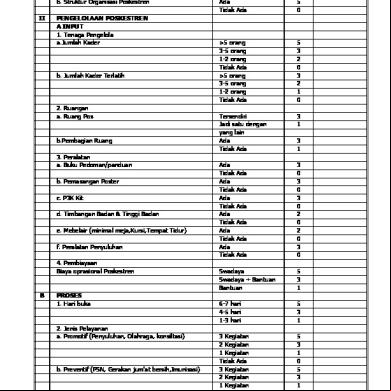
Strata Poskestren 3d1i4p
April 2020 23
Penilaian Strata Desa Siaga.docx 72t2t
July 2020 0More Documents from "Hafidz Dezulfakar" i4v3l
Strata 3y5to
February 2021 0
Install Petrel 2013 4s6c59
December 2019 19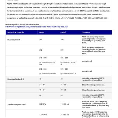
Assab Steels 709m Machinery Steel 1i5t4d
November 2019 137
Cheat Gta San Andreas For Android 4z186h
November 2019 1,168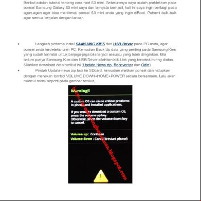
Cara Root Dan Unroot Samsung Galaxy S3 Mini Gt 1m33a
November 2019 61