Spss Intro 6z6o2j
This document was ed by and they confirmed that they have the permission to share it. If you are author or own the copyright of this book, please report to us by using this report form. Report r6l17
Overview 4q3b3c
& View Spss Intro as PDF for free.
More details 26j3b
- Words: 2,205
- Pages: 83
TRAINING SPSS 20 KONSENTRASI EPIDEMIOLOGI PASCA SARJANA UNHAS 2013
PROFESSIONAL
DYNAMIC
ABSTRACT
CREATIVE
SOPHISTICATED
MODERN
The Four Windows: Data editor Output viewer Syntax editor Script window
SPSS Files and Extensions • Portable file --
.por
• Data file --
.sav
• Output file --
.spo
• Syntax file --
.sps
5/6/2011
www.ssric.org
The Four Windows: Data Editor • Data Editor Spreadsheet-like system for defining, entering, editing, and displaying data. Extension of the saved file will be “sav.”
The Four Windows: Output Viewer • Output Viewer Displays output and errors. Extension of the saved file will be “spv.”
The Four Windows: Syntax editor • Syntax Editor Text editor for syntax composition. Extension of the saved file will be “sps.”
The Four Windows: Script Window • Script Window Provides the opportunity to write full-blown programs, in a BASIC-like language. Text editor for syntax composition. Extension of the saved file will be “sbs.”
Data View
5/6/2011
www.ssric.org
Variable View
Variable Names Variable Labels Value Labels
MissingValues
5/6/2011
www.ssric.org
The basics of managing data files
Opening SPSS • Start → All Programs → SPSS Inc→ SPSS 20 → SPSS 20
Opening SPSS • The default window will have the data editor • There are two sheets in the window: 1. Data view 2. Variable view
Data View window • The Data View window This sheet is visible when you first open the Data Editor and this sheet contains the data • Click on the tab labeled Variable View
Click
Variable View window • This sheet contains information about the data set that is stored with the dataset • Name – The first character of the variable name must be alphabetic – Variable names must be unique, and have to be less than 64 characters. – Spaces are NOT allowed.
Variable View window: Type • Type – Click on the ‘type’ box. The two basic types of variables that you will use are numeric and string. This column enables you to specify the type of variable.
Variable View window: Width • Width – Width allows you to determine the number of characters SPSS will allow to be entered for the variable
Variable View window: Decimals • Decimals – Number of decimals – It has to be less than or equal to 16
3.14159265
Variable View window: Label • Label – You can specify the details of the variable – You can write characters with spaces up to 256 characters
Variable View window: Values • Values – This is used and to suggest which numbers represent which categories when the variable represents a category
Defining the value labels • Click the cell in the values column as shown below • For the value, and the label, you can put up to 60 characters. • After defining the values click add and then click OK.
Click
Practice 1 • How would you put the following information into SPSS? Name JAUNITA SALLY DONNA SABRINA JOHN MARK ERIC BRUCE
Gender 2 2 2 2 1 1 1 1
Height 5.4 5.3 5.6 5.7 5.7 6 6.4 5.9
Value = 1 represents Male and Value = 2 represents Female
Practice 1 (Solution Sample)
Click
Click
Saving the data • To save the data file you created simply click ‘file’ and click ‘save as.’ You can save the file in different forms by clicking “Save as type.”
Click
Transforming data • Click ‘Transform’ and then click ‘Compute Variable…’
Transforming data (cont’d) • Example: Adding a new variable named ‘lnheight’ which is the natural log of height – Type in lnheight in the ‘Target Variable’ box. Then type in ‘ln(height)’ in the ‘Numeric Expression’ box. Click OK
Click
Transforming data (cont’d) • A new variable ‘lnheight’ is added to the table
Practice 3 • Create a new variable named “sqrtheight” which is the square root of height. • Answer
Transforming Data • We can transform variables by recoding, i.e., combining categories in an existing variable into fewer categories. • We can also transform variables by creating new variables out of existing variables. • We can select particular cases and analyze only these cases.
5/6/2011
www.ssric.org
Recoding into Different Variables
• Click on Transform > Recode > Into different variables.
• Select the variable you want to recode. age Start by giving the new variable a new name (age1) Click on Change Click on Old and New Values 5/6/2011
www.ssric.org
Recoding age into AGE1 • Use “Range” (fourth option down) to recode as follows. to click on “Add” after entering each recode. – 18 to 29 = 1 – 30 to 49 = 2 – 50 to 69 = 3 – 70 to 89 = 4 • Click Continue And then OK.
Assign Value Labels to the Four Categories of AGE1 • Select the Variable View tab. • Scroll down the variables to age1 (at the bottom of the list). • In the Values column of age1 click on the small gray box. • Enter the first value followed by its label. Click Add.
• Enter remaining 3
18 to 29 = 1 30 to 49 = 2 50 to 69 = 3 values.70 to 89 = 4
Exercises for Recoding • Now recode income06 and call the new variable income2 • This time use 8 categories: under $10K, $10K to under $20K, $20K to under $30K, $30K to under $40K, $40K to under $50K, $50K to under $60K, $60K to under $75K, and $75K and over
• Add the value labels • Run a frequency distribution for income2 and check to make sure that you recoded it correctly by comparing the unrecoded and recoded frequency distributions
Creating a New Variable with Compute • Let’s create a new variable and call it timewaste which is the percentage of relaxation time (hrsrelax) devoted to watching TV (tvhours) • Click on Transform > Compute • Enter the new variable name (timewaste) into the Target Variable box. • Enter the formula for this new variable (100*tvhours/hrsrelax) into the Numeric 5/6/2011 Expression box. www.ssric.org
Caution! • If, for any case, any of the variables used to create a new variable has a missing value, the new variable will automatically be assigned a missing value as well.
5/6/2011
www.ssric.org
Exercise for Compute • The data file includes indexes of socio-economic status for respondents (sei), their mothers (masei) and their fathers (pasei).
• Create an index of mobility by subtracting sei from an average of masei and pasei.
5/6/2011
www.ssric.org
Using Select Cases to Select Specific Cases for Analysis • Let’s select only Protestants for further analysis. • Click on Data > Select Cases. • Click on “If condition is satisfied” and then on the “If” button below it.
Using Select Cases to Select Specific Cases for Analysis • Select the variable relig ( R’s RELIGEOUS PREFERENCE) and move it into the box on the right. • In this box, enter the expression relig = 1. • Click on Continue and on OK.
5/6/2011
www.ssric.org
Using Select Cases to Select Specific Cases for Analysis • Note all cases not accepted are crossed out on the left.
• Again click on Data > Select Cases. • Click on “all” and then OK. 5/6/2011
www.ssric.org
Important Note on Using
Select Cases • When you are finished using Select Cases and want to revert to using all the cases be sure to click on Data > Select Cases and select All cases. Then click on OK • If you don’t do this, you will continue to use only those cases you last selected
5/6/2011
www.ssric.org
Exercises for Select Cases • Select all males (1 on the variable sex) and do a frequency distribution for the variable partyid (political party identification) • Now select all females (2 on the variable sex) and run a frequency distribution for partyid • Is there a “gender gap” in party identification. How large is it? • Note: same thing could have been done with Crosstabs 5/6/2011
www.ssric.org
Univariate Analysis • Now that we know how to open existing files and transform variables, we’re ready to begin analyzing data • Univariate analysis refers to analyzing variables one-at-a-time
5/6/2011
www.ssric.org
Types of Univariate Analysis Procedures • Frequencies
• Descriptives • Explore
5/6/2011
www.ssric.org
Frequencies • Go to: Analyze > Descriptive Statistics > Frequencies
• Select age1 and age
• Notice Statistics and Charts buttons at upper right and Display frequencies tables check-box at lower left
5/6/2011
www.ssric.org
Frequencies: Statistics • Click on Statistics • Select the statistics you want • Click on Continue
5/6/2011
www.ssric.org
Frequencies: Charts • Click on Charts • Select Histograms and check With normal curve • Click on Continue • Click on OK
5/6/2011
www.ssric.org
Frequencies: Output - Tables
5/6/2011
www.ssric.org
Frequencies: Output - Statistics
5/6/2011
www.ssric.org
Frequencies: Output - Charts
5/6/2011
www.ssric.org
Exercises for Frequencies • Run frequency distributions for hrsrelax and tvhours with appropriate statistics and charts • Run frequency distributions for cappun, grass, and gunlaw with appropriate statistics and charts
5/6/2011
www.ssric.org
Descriptives • Click on Analyze > Descriptive Statistics > Descriptives
• Select age and educ
• Click on Options and select the statistics you want and then click on Continue and OK
5/6/2011
Descriptives (continued)
Descriptive Statistics N age AGE OF RESPONDENT educ HIGHEST YEAR OF SCHOOL COMPLETED Valid N (listwise)
5/6/2011
Minimum
Maximum
Mean
Std. Deviation
4496
18
89
45.34
16.546
4502
0
20
13.25
3.213
4486
www.ssric.org
Exercise for Descriptives • Use Descriptives to compute the following statistics for hrs1 (hours worked per week) – Mean – Standard deviation – Variance – Skewness – Kurtosis
5/6/2011
www.ssric.org
More Exercises for Descriptives • Use Descriptives to compute the mean for educ, maeduc, and paeduc • Who has the most education – respondents or their parents? • Who has the most education – mothers or fathers?
5/6/2011
www.ssric.org
Explore • Click on Analyze > Descriptive Statistics > Explore
• Select hrs1 and put it in the Dependent List • In the Display box on the lower left, click on Both 5/6/2011
www.ssric.org
Explore (continued) • Click on Statistics • Select the statistics you want
• Click on Continue
5/6/2011
www.ssric.org
Explore (continued) • Click on Plots • Select the plots you want • Click on Continue • Click on OK
Explore (continued) Descriptives Statistic hrs1 NUMBER OF HOURS WORKED LAST WEEK
Std. Error
Mean
42.13
95% Confidence Interval for Lower Bound
41.59
Mean
Upper Bound
42.66
5% Trimmed Mean
41.90
Median
40.00
Variance Std. Deviation
208.271 14.432
Minimum
1
Maximum
89
Range
88
Interquartile Range
12
Skewness Kurtosis
.272
.272
.046
1.243
.092
Explore (continued)
Descriptives Statistic hrs1 NUMBER OF HOURS WORKED LAST WEEK
Std. Error
Mean
42.13
95% Confidence Interval for Lower Bound
41.59
Mean
Upper Bound
42.66
5% Trimmed Mean
41.90
Median
40.00
Variance Std. Deviation
208.271 14.432
Minimum
1
Maximum
89
Range
88
Interquartile Range
12
Skewness Kurtosis
.272
.272
.046
1.243
.092
Graphs: Bar Charts • Click on
5/6/2011
Graphs > Legacy Dialogs > Bar
www.ssric.org
Graphs: Bar Charts (continued)
Click on “Simple”
Click on “Define”
5/6/2011
www.ssric.org
Graphs: Bar Charts (continued)
Click on “% of cases”
Drag or move marital to second box on right
Click on “OK”
5/6/2011
www.ssric.org
Graphs: Pie Charts • Click on
5/6/2011
Graphs > Legacy Dialogs > Pie
www.ssric.org
Graphs: Pie Charts • Click on “Define”
5/6/2011
www.ssric.org
Graphs: Pie Charts • Click on “% of cases”
• Drag or move marital to second box on right • Click on “OK”
5/6/2011
www.ssric.org
Graphs: Box and Whiskers Plots • Click on
5/6/2011
Graphs > Legacy Dialogs > Boxplots
www.ssric.org
Graphs: Box and Whiskers Plots (continued) • Drag or move tvhours to first box on right • Drag or move degree to second box on right • Click on OK
5/6/2011
www.ssric.org
Graphs: Box and Whiskers Plots (continued)
Extreme Values (>3.0 X IQR) Outliers (1.5 – 3.0 IQR)
Median
5/6/2011
Box (IQR)
Whiskers (< 1.5 X IQR)
www.ssric.org
Graphs: Scatterplots • Click on
5/6/2011
Graphs > Legacy Dialogs > Scatterplot
www.ssric.org
Graphs: Scatterplots (continued) • Click on “Simple Scatter” • Click on “Define”
5/6/2011
www.ssric.org
Graphs: Scatterplots (continued)
• Drag or move maeduc to first box on right
• Drag or move paeduc to second box on right • Click on OK
• Double-click on chart • Click on “Elements” and “Fit Line at Total” 5/6/2011
www.ssric.org
Graphs: Histograms • Click on
5/6/2011
Graphs > Legacy Dialogs > Histogram
www.ssric.org
Graphs: Histograms (continued) • Drag or move realinc to first box on right • Check “Display normal curve” • Click on OK
5/6/2011
www.ssric.org
10 MINUTE BREAK!
5/6/2011
www.ssric.org
The basic analysis
The basic analysis of SPSS that will be introduced in this class • Frequencies – This analysis produces frequency tables showing frequency counts and percentages of the values of individual variables.
• Descriptives – This analysis shows the maximum, minimum, mean, and standard deviation of the variables
• Linear regression analysis – Linear Regression estimates the coefficients of the linear equation
Frequencies • Click ‘Analyze,’ ‘Descriptive statistics,’ then click ‘Frequencies’
Frequencies • Click gender and put it into the variable box. • Click ‘Charts.’ • Then click ‘Bar charts’ and click ‘Continue.’
Click
Click
Frequencies • Finally Click OK in the Frequencies box.
Click
Questions?
Related Documents 171j1w

Spss Intro 6z6o2j
November 2021 0
Spss 4q4z2w
January 2021 0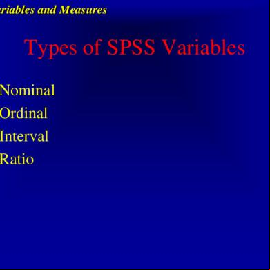
Spss 4q4z2w
October 2021 0
Spss 4q4z2w
September 2022 0
Spss 4q4z2w
December 2019 54
Spss 4q4z2w
October 2021 0More Documents from "Ardiani " 1s4l3s
Spss Intro 6z6o2j
November 2021 0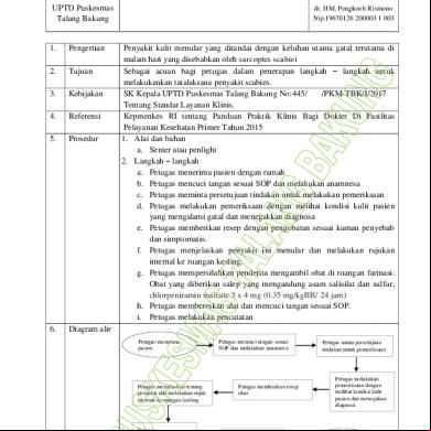
Sop 144 Penyakit Pkmtbk Watermark 5ri72
June 2020 4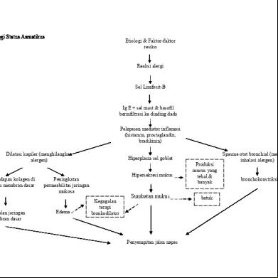
Patofis Status Asmatikus 29443x
November 2019 59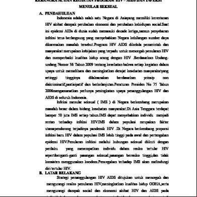
Kerangka Acuan Hiv Aids Dan Ims 5r6m2m
April 2020 25
Data Bpjs Dan Penduduk 2019 34612e
January 2021 0