5 Double And Triple Integrals.pdf 3y6t4x

MULTIVARIABLE AND VECTOR ANALYSIS W W L CHEN c

W W L Chen, 1997, 2008.

This chapter is available free to all individuals, on the understanding that it is not to be used for financial gain, and may be ed and/or photocopied, with or without permission from the author. However, this document may not be kept on any information storage and retrieval system without permission from the author, unless such system is not accessible to any individuals other than its owners.

Chapter 5 DOUBLE AND TRIPLE INTEGRALS

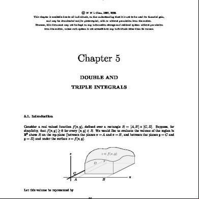
5.1. xxxxx Introduction Consider a real valued function f (x, y), defined over a rectangle R = [A, B] × [C, D]. Suppose, for simplicity, that f (x, y) ≥ 0 for every (x, y) ∈ R. We would like to evaluate the volume of the region in R3 above R on the xy-plane (between the planes x = A and x = B, and between the planes y = C and y = D) and under the surface z = f (x, y).

z

z = f (x, y) D

y

C A

B

x

Let this volume be represented by ZZ R

f (x, y) dxdy.

The purpose of this chapter is to investigate the properties of this “integral”. Chapter 5 : Double and Triple Integrals

page 1 of 21

xxxxx c

Multivariable and Vector Analysis

W W L Chen, 1997, 2008

We shall first of all take a very cavalier approach to the problem. Consider the simpler case of a function f (x) defined over an interval [A, B]. Suppose, for simplicity, that f (x) ≥ 0 for every x ∈ [A, B].

y = f (x)

A

x

x+∆x

B

Let us split the interval [A, B] into a large number of very short intervals. Consider now one such interval [x, x + ∆x], where ∆x is very small. Then the region in R2 above the interval [x, x + ∆x] on the x-axis and under the curve y = f (x) is roughly a rectangle with base ∆x and height f (x), and so has area roughly equal to f (x)∆x. Hence the area of the region in R2 above the interval [A, B] on the x-axis and under the curve y = f (x) is roughly X

f (x)∆x,

∆x

where the summation is over all these very short intervals making up the interval [A, B]. As ∆x → 0, we have, with any luck, X

f (x)∆x →

∆x

Z

B

A

f (x) dx.

We next extend this approach to the problem of finding the volume of an object in 3-space. Consistent with our lack of rigour so far, the following seems plausible. CAVALIERI’S PRINCIPLE. Suppose that S is a solid in 3-space, and that for u ∈ [α, β], Pu is a family of parallel planes perpendicular to the direction of u and such that the solid S lies between the planes Pα and Pβ . Suppose further that for every u ∈ [α, β], the area of the intersection of S with the plane Pu is given by a(u). Then the volume of S is given by xxxxx

Z

β

α

a(u) du.

Let us now apply Cavalieri’s principle to our original problem. For every u ∈ [A, B], let Pu denote the plane x = u. Pu

1 A Chapter 5 : Double and Triple Integrals

u

B

x

page 2 of 21

c

Multivariable and Vector Analysis

W W L Chen, 1997, 2008

Clearly the region in question lies between the planes PA and PB . On the other hand, if a(u) denotes the area of the intersection between the region in question and the plane x = u, then Z D f (u, y) dy. a(u) = C

By Cavalieri’s principle, the volume of the region in question is now given by ! ! Z B Z D Z B Z B Z D f (x, y) dy dx. f (u, y) dy du = a(u) du = A

C

A

C

A

Similarly, for every u ∈ [C, D], let Pu denote the plane y = u. Clearly the region in question lies between the planes PC and PD . On the other hand, if a(u) denotes the area of the intersection between the region in question and the plane y = u, then Z B a(u) = f (x, u) dx. A

By Cavalieri’s principle, the volume of the region in question is now given by ! ! Z D Z D Z B Z D Z B a(u) du = f (x, u) dx du = f (x, y) dx dy. C

C

A

C

A

We therefore conclude that, with any luck, ZZ R

f (x, y) dxdy =

Z

B

Z

A

D

! f (x, y) dy dx =

C

Z

D

C

Z

B

A

! f (x, y) dx dy.

(1)

Unfortunately, the identity (1) does not hold all the time. Example 5.1.1. Consider the function f : [0, 1] × [0, 1] → R, given by 1 if x is rational, f (x, y) = 2y if x is irrational, Then Z 1    Z 1 dy = 1  0 f (x, y) dy = Z 1  0   2y dy = 1  0

if x is rational, if x is irrational,

so that Z

1

1

Z

0



f (x, y) dy dx = 1.

0

On the other hand, the integral 1

Z 0

f (x, y) dx

does not exist except when y = 1/2, so Z 0

1

Z 0

1

f (x, y) dx dy

does not exist. Chapter 5 : Double and Triple Integrals

page 3 of 21

c

Multivariable and Vector Analysis

W W L Chen, 1997, 2008

5.2. Double Integrals over Rectangles Suppose that the function f : R → R2 is bounded in R, where R = [A, B]×[C, D] is a rectangle. Suppose further that ∆ : A = x0 < x1 < x2 < . . . < xn = B, C = y0 < y1 < y2 < . . . < ym = D is a dissection of the rectangle R = [A, B] × [C, D]. Definition. The sum s(∆) =

n X m X (xi − xi−1 )(yj − yj−1 ) i=1 j=1

min

(x,y)∈[xi−1 ,xi ]×[yj−1 ,yj ]

f (x, y)

is called the lower Riemann sum of f (x, y) corresponding to the dissection ∆. Definition. The sum S(∆) =

n X m X

(xi − xi−1 )(yj − yj−1 )

i=1 j=1

max

(x,y)∈[xi−1 ,xi ]×[yj−1 ,yj ]

f (x, y)

is called the upper Riemann sum of f (x, y) corresponding to the dissection ∆. Remark. xxxxx Strictly speaking, the above definitions are invalid, since the minimum or maximum may not exist. The correct way is to replace the minimum and maximum with infimum and supremum respectively. However, since we have not discussed infimum and supremum, we shall be somewhat economical with the truth and simply use minimum and maximum. Definition. Suppose that for every i = 1, . . . , n and j = 1, . . . , m, the point (ξij , ηij ) lies in the rectangle [xi−1 , xi ] × [yj−1 , yj ]. D yj

(ξij , ηij )

yj−1 C A

xi−1

xi

B

Then the sum n X m X (xi − xi−1 )(yj − yj−1 )f (ξij , ηij ) i=1 j=1

is called a Riemann sum of f (x, y) corresponding to the dissection ∆. Remarks. (1) It is clear that min

(x,y)∈[xi−1 ,xi ]×[yj−1 ,yj ] Chapter 5 : Double and Triple Integrals

f (x, y) ≤ f (ξij , ηij ) ≤

max

(x,y)∈[xi−1 ,xi ]×[yj−1 ,yj ]

f (x, y). page 4 of 21

c

Multivariable and Vector Analysis

W W L Chen, 1997, 2008

It follows that every Riemann sum is bounded below by the corresponding lower Riemann sum and bounded above by the corresponding upper Riemann sum; in other words, s(∆) ≤

n X m X

(xi − xi−1 )(yj − yj−1 )f (ξij , ηij ) ≤ S(∆).

i=1 j=1

(2) It can be shown that for any two dissections ∆0 and ∆00 of the rectangle R = [A, B] × [C, D], we have s(∆0 ) ≤ S(∆00 ); in other words, a lower Riemann sum can never exceed an upper Riemann sum. Definition. We say that ZZ R

f (x, y) dxdy = L

if, given any > 0, there exists a dissection ∆ of R = [A, B] × [C, D] such that L − < s(∆) ≤ S(∆) < L + . In this case, we say that the function f (x, y) is Riemann integrable over the rectangle R = [A, B]×[C, D] with integral L. Remark. In other words, if the lower Riemann sums and upper Riemann sums can get arbitrarily close, then their common value is the integral of the function. The following result follows easily from our definition. The proof is left as an exercise. THEOREM 5A. Suppose that the functions f : R → R and g : R → R are Riemann integrable over the rectangle R = [A, B] × [C, D]. (a) Then the function f + g is Riemann integrable over R, and ZZ R

ZZ

(f (x, y) + g(x, y)) dxdy =

R

f (x, y) dxdy +

ZZ R

g(x, y) dxdy;

(b) On the other hand, for any c ∈ R, the function cf is Riemann integrable over R, and ZZ R

cf (x, y) dxdy = c

ZZ R

f (x, y) dxdy.

(c) Suppose further that f (x, y) ≥ g(x, y) for every (x, y) ∈ R. Then ZZ R

f (x, y) dxdy ≥

ZZ R

g(x, y) dxdy.

We also state without proof the following result. THEOREM 5B. Suppose that Q = R1 ∪ . . . ∪ Rp is a rectangle, where, for k = 1, . . . , p, the rectangles Rk = [Ak , Bk ] × [Ck , Dk ] are pairwise dist, apart possibly from boundary points. Suppose further that the function f : Q → R is bounded in Q. Then f is Riemann integrable over Q if and only if it is Riemann integrable over Rk for every k = 1, . . . , p. In this case, we also have ZZ Q Chapter 5 : Double and Triple Integrals

f (x, y) dxdy =

p ZZ X k=1

Rk

f (x, y) dxdy. page 5 of 21

c

Multivariable and Vector Analysis

W W L Chen, 1997, 2008

5.3. Conditions for Integrability The following important result will be discussed in Section 5.5. THEOREM 5C. (FUBINI’S THEOREM) Suppose that the function f : R → R is continuous in the rectangle R = [A, B]×[C, D]. Then f is Riemann integrable over R. Furthermore, the identity (1) holds. Example 5.3.1. Consider the integral ZZ R

(x2 + y 2 ) dxdy,

where R = [0, 2] × [0, 1] is a rectangle. Since the function f (x, y) = x2 + y 2 is continuous in R, the integral exists by Fubini’s theorem. Furthermore, Z 2 Z 2 Z 1 1 10 dx = . x2 + (x2 + y 2 ) dy dx = 3 3 0 0 0 On the other hand, 1

Z

Z

0

0

2

Z (x2 + y 2 ) dx dy =

1



0

8 10 + 2y 2 dy = . 3 3

By Fubini’s theorem, ZZ R

(x2 + y 2 ) dxdy =

10 . 3

Example 5.3.2. Consider the integral ZZ R

sin x cos y dxdy,

where R = [0, π] × [−π/2, π/2] is a rectangle. Since the function f (x, y) = sin x cos y is continuous in R, the integral exists by Fubini’s theorem. Furthermore, ! Z π Z π/2 Z π sin x cos y dy dx = 2 sin x dx = 4. 0

−π/2

0

On the other hand, Z

π/2

Z

−π/2

0

π



sin x cos y dx dy =

Z

π/2

−π/2

2 cos y dy = 4.

By Fubini’s theorem, ZZ R

sin x cos y dxdy = 4.

5.4. Double Integrals over Special Regions The purpose of this section is to study Riemann integration over regions R which are not necessarily rectangles of the form [A, B] × [C, D]. Our argument hinges on the following generalization of Fubini’s theorem. Chapter 5 : Double and Triple Integrals

page 6 of 21

c

Multivariable and Vector Analysis

W W L Chen, 1997, 2008

xxxxx Definition. Consider the rectangle R = [A, B] × [C, D]. A set of the form {(x, φ(x)) : x ∈ [A, B]} ⊆ R is said to be a curve of type 1 in R if the function φ : [A, B] → R is continuous in the interval [A, B]. D y = φ(x) C A

xxxxx

B

A set of the form {(ψ(y), y) : y ∈ [C, D]} ⊆ R is said to be a curve of type 2 in R if the function ψ : [C, D] → R is continuous in the interval [C, D]. D x = ψ(y) C A

B

THEOREM 5D. Suppose that the function f : R → R is bounded in the rectangle R = [A, B] × [C, D]. Suppose further that f is continuous in R, except possibly at points contained in a finite number of curves of type 1 or 2 in R. Then f is Riemann integrable over R. Furthermore, if the integral D

Z

C

f (x, y) dy

exists for every x ∈ [A, B], then the integral Z

B

D

Z

A

C

! f (x, y) dy dx

exists, and ZZ R

f (x, y) dxdy =

Z

B

A

Z

D

C

! f (x, y) dy dx.

Similarly, if the integral Z

B

A Chapter 5 : Double and Triple Integrals

f (x, y) dx 1

page 7 of 21

c

Multivariable and Vector Analysis

W W L Chen, 1997, 2008

exists for every y ∈ [C, D], then the integral Z

D

Z

B

A

C

! f (x, y) dx dy

exists, and ZZ R

f (x, y) dxdy =

Z

D

Z

B

A

C

! f (x, y) dx dy.

Thus, the identity (1) holds if all the integrals exist. In view of Theorem 5D, we can now study integrals over some special regions. xxxxx Definition. Suppose that φ1 : [A, B] → R and φ2 : [A, B] → R are continuous in the interval [A, B]. Suppose further that φ1 (x) ≤ φ2 (x) for every x ∈ [A, B]. Then we say that S = {(x, y) ∈ R2 : x ∈ [A, B] and φ1 (x) ≤ y ≤ φ2 (x)}

(2)

is an elementary region of type 1. D

y = φ2 (x) y = φ1 (x)

C A

B

Suppose now that S is an elementary region of type 1, of the form (2). Since φ1 : [A, B] → R and φ2 : [A, B] → R are continuous in [A, B], there exist C, D ∈ R such that C ≤ φ1 (x) ≤ φ2 (x) ≤ D for every x ∈ [A, B]. It follows that S ⊆ R, where R = [A, B] × [C, D]. Suppose that the function f : S → R is continuous in S. Then it is bounded in S. Hence the function f ∗ : R → R, defined by f (x, y) if (x, y) ∈ S, ∗ f (x, y) = 0 if (x, y) 6∈ S, is bounded in R. Furthermore, it is continuous in R, except possibly at points contained in two curves of type 1 in R. It follows from Theorem 5D that f ∗ is Riemann integrable over R. We can now define ZZ ZZ f (x, y) dxdy = f ∗ (x, y) dxdy. S

R

On the other hand, for any x ∈ [A, B], the function f ∗ (x, y) = f (x, y) is a continuous function of y in the interval [φ1 (x), φ2 (x)]. Also, f ∗ (x, y) = 0 for every y ∈ [C, φ1 (x)) ∪ (φ2 (x), D]. Hence Z

D

C

f ∗ (x, y) dy =

Z

!

Z

φ2 (x)

φ1 (x)

f (x, y) dy,

and so Z

B

A

Z

D

C

Chapter 5 : Double and Triple Integrals

∗

f (x, y) dy dx =

B

A

Z

φ2 (x)

φ1 (x)

! f (x, y) dy dx. page 8 of 21

c

Multivariable and Vector Analysis

W W L Chen, 1997, 2008

We have proved the following result. THEOREM 5E. Suppose that S is an elementary region of type 1, of the form (2). Suppose further that the function f : S → R is continuous in S. Then ZZ S

B

Z

f (x, y) dxdy =

φ2 (x)

Z

φ1 (x)

A

! f (x, y) dy dx.

xxxxx Definition. Suppose that ψ1 : [C, D] → R and ψ2 : [C, D] → R are continuous in the interval [C, D]. Suppose further that ψ1 (y) ≤ ψ2 (y) for every y ∈ [C, D]. Then we say that S = {(x, y) ∈ R2 : y ∈ [C, D] and ψ1 (y) ≤ x ≤ ψ2 (y)}

(3)

is an elementary region of type 2. D x = ψ2 (y)

x = ψ1 (y) C A

B

Analogous to Theorem 5E, we have the following result. THEOREM 5F. Suppose that S is an elementary region of type 2, of the form (3). Suppose further that the function f : S → R is continuous in S. Then ZZ S

xxxxx

D

Z

f (x, y) dxdy =

Z

C

ψ2 (y)

ψ1 (y)

! f (x, y) dx dy.

Example 5.4.1. The function f (x, y) = x2 + y 2 is continuous in the triangle S with vertices (0, 0), (1, 0) and (1, 1). It is easy to see that S is an elementary region of type 1, of the form S = {(x, y) ∈ R2 : x ∈ [0, 1] and 0 ≤ y ≤ x}. 1 y=x S y=0

1

By Theorem 5E, ZZ

2

S

2

(x + y ) dxdy =

Chapter 5 : Double and Triple Integrals

Z 0

1

Z 0

x

2

2



(x + y ) dy dx =

Z 0

1

4 3 1 x dx = . 3 3 page 9 of 21

c

Multivariable and Vector Analysis

W W L Chen, 1997, 2008

xxxxx On the other hand, it is also easy to see that S is an elementary region of type 2, of the form S = {(x, y) ∈ R2 : y ∈ [0, 1] and y ≤ x ≤ 1}. 1 x=y

x=1

S 1 By Theorem 5F, ZZ

2

S

2

(x + y ) dxdy =

Z

1

0

Z y

1

2



2

(x + y ) dx dy =

Z

1



0

1 4 3 1 2 + y − y dy = . 3 3 3

xxxxx Example 5.4.2. The function f (x, y) = sin x cos y is continuous in the parallelogram S with vertices (π, 0), (π, π) and (0, ±π/2). It is easy to see that S is an elementary region of type 1, of the form n x πo x π . S = (x, y) ∈ R2 : x ∈ [0, π] and − ≤ y ≤ + 2 2 2 2 π π/2

S π

−π/2 By Theorem 5E, ZZ S

π

x π 2+2

!

π

x π x π sin x sin + − sin − dx x π 2 2 2 2 0 0 2−2 Z π x π x π x π x π = sin x sin cos + cos sin − sin cos + cos sin dx 2 2 2 2 2 2 2 2 0 Z π Z π x x x 8 =2 sin x cos dx = 4 sin cos2 dx = . 2 2 2 3 0 0

sin x cos y dxdy =

Z

Z

sin x cos y dy dx =

Z

On the other hand, it is also easy to see that S is an elementary region of type 2, of the form n h π i o S = (x, y) ∈ R2 : y ∈ − , π and ψ1 (y) ≤ x ≤ ψ2 (y) , 2 where ψ1 (y) =



0 2y − π

if y ∈ [−π/2, π/2], if y ∈ [π/2, π],

and

ψ2 (y) =



2y + π π

if y ∈ [−π/2, 0], if y ∈ [0, π].

1 Chapter 5 : Double and Triple Integrals

page 10 of 21

c

Multivariable and Vector Analysis

W W L Chen, 1997, 2008

By Theorem 5F, ZZ sin x cos y dxdy S

=

Z

=

Z

=

Z

0

0

−π/2 0

−π/2 0

−π/2

=2− =2+ =2+ =2+

2y+π

Z

Z

π/2

Z sin x cos y dx dy +

cos y dy + 2

−π/2 Z 0 −π/2 Z 0 −π/2 Z 0 −π/2

Z

π/2

0

cos y dy +

Z

π

0

0

(cos y − cos(2y + π) cos y) dy +

0

Z

π/2

Z 0

π

π/2

Z

π

π/2

(1 − 2 sin y) cos y dy − Z

π

π/2

Z

cos y dy − Z

Z

π/2

0

−π/2 π

π/2

π

Z

π

sin x cos y dx dy

2y−π

(cos y + cos(2y − π) cos y) dy

cos(2y + π) cos y dy +

Z

π

π/2

cos(2y − π) cos y dy

(cos 2y cos π + sin 2y sin π) cos y dy

cos 2y cos y dy

2

cos y dy −

π

π/2

2 cos y dy +

(cos 2y cos π − sin 2y sin π) cos y dy + cos 2y cos y dy −

Z sin x cos y dx dy +

Z

π

π/2

cos y dy − 2

(1 − 2 sin2 y) cos y dy

Z

0

−π/2

sin2 y cos y dy + 2

Z

π

π/2

sin2 y cos y dy =

8 . 3

Note that the calculation is much simpler if we think of S as an elementary region of type 1. We can extend our study further. Suppose that T = S1 ∪ . . . ∪ Sp is a finite region in R2 , where, for every k = 1, . . . , p, Sk is an elementary region of type 1 or 2. Suppose further that S1 , . . . , Sp are pairwise dist, apart possibly from boundary points. Then we can define ZZ

xxxxx

T

f (x, y) dxdy =

p ZZ X k=1

Sk

f (x, y) dxdy,

provided that every integral on the right hand side exists. Example 5.4.3. Consider the finite region T bounded by the four lines y = x, y = −x, y = 2x − 2 and y = 2 − 2x and with vertices (0, 0), (2, −2), (1, 0) and (2, 2). 2

S1 S2

2

−2 Note that T = S1 ∪ S2 , where S1 is the triangle with vertices (0, 0), (1, 0) and (2, 2) and S2 is the triangle with vertices (0, 0), (1, 0) and (2, −2). It is easy to see that S1 and S2 are dist, apart from boundary points. Clearly the function f (x, y) = x + y 2 is continuous in T , and so continuous in S1 and S2 . Hence ZZ ZZ ZZ (x + y 2 ) dxdy = (x + y 2 ) dxdy + (x + y 2 ) dxdy. T

Chapter 5 : Double and Triple Integrals

S1

S2

page 11 of 21

c

Multivariable and Vector Analysis

W W L Chen, 1997, 2008

To study the first integral on the right hand side, it is easier to interpret S1 as an elementary region of type 2, of the form n yo S1 = (x, y) ∈ R2 : y ∈ [0, 2] and y ≤ x ≤ 1 + . 2 Then ZZ

(x + y ) dxdy =

Z

=

Z

2

S1

2

Z

0

1+ y2

y 2



0

! 2

(x + y ) dx dy =

2

Z 0

1 y 2 y 2 1 2 1+ y − y − y 3 dy + 1+ 2 2 2 2

5 1 1 1 5 + y + y 2 − y 3 dy = . 2 2 8 2 3

To study the second integral on the right hand side, it is again easier to interpret S2 as an elementary region of type 2, of the form n yo . S2 = (x, y) ∈ R2 : y ∈ [−2, 0] and − y ≤ x ≤ 1 − 2 Then ZZ S2

(x + y ) dxdy =

Z

=

Z

2

0

Z

−2 0

−2

1− y2

−y



! 2

(x + y ) dx dy =

0

1 y 2 y 2 1 2 1− + 1− y − y + y 3 dy 2 2 2 2 −2

Z

1 1 5 1 5 − y + y 2 + y 3 dy = . 2 2 8 2 3

Hence xxxxx ZZ T

(x + y 2 ) dxdy =

10 . 3

Example 5.4.4. Consider the region T in the first quadrant between the two circles of radii 1 and 2 and centred at (0, 0). 2 S1 1 S2 1

2

Note that T = S1 ∪ S2 , where S1 = {(x, y) ∈ R2 : x ∈ [0, 1] and (1 − x2 )1/2 ≤ y ≤ (4 − x2 )1/2 } and S2 = {(x, y) ∈ R2 : x ∈ [1, 2] and 0 ≤ y ≤ (4 − x2 )1/2 } are elementary regions of type 1 and dist, apart from boundary points. The function f (x, y) = x2 +y 2 is clearly continuous in T , and so continuous in S1 and S2 . Hence ZZ ZZ ZZ (x2 + y 2 ) dxdy = (x2 + y 2 ) dxdy + (x2 + y 2 ) dxdy. T

Chapter 5 : Double and Triple Integrals

S1

S2

page 12 of 21

c

Multivariable and Vector Analysis

W W L Chen, 1997, 2008

We have ZZ

2

S1

2

(x + y ) dxdy =

1

Z

(4−x2 )1/2

Z

0

(1−x2 )1/2

! 2

2

(x + y ) dy dx

1

1 1 2 2 1/2 2 3/2 2 2 1/2 2 3/2 x (4 − x ) + (4 − x ) − x (1 − x ) − (1 − x ) = dx 3 3 0 Z Z Z Z 2 1 2 1 1 2 1 2 4 1 (4 − x2 )1/2 dx + x (4 − x2 )1/2 dx − (1 − x2 )1/2 dx − x (1 − x2 )1/2 dx = 3 0 3 0 3 0 3 0 Z

and ZZ

2

S2

2

(x + y ) dxdy = =

2

Z 1



Z

2

(4−x2 )1/2

Z

1

0

! 2

2

(x + y ) dy dx

Z Z 1 4 2 2 2 2 (4 − x2 )1/2 dx + x (4 − x2 )1/2 dx. x2 (4 − x2 )1/2 + (4 − x2 )3/2 dx = 3 3 1 3 1

Hence ZZ (x2 + y 2 ) dxdy T

=

4 3

Z 0

2

(4 − x2 )1/2 dx +

2 3

Z 0

2

x2 (4 − x2 )1/2 dx −

1 3

Z

1

0

(1 − x2 )1/2 dx −

2 3

Z 0

1

x2 (1 − x2 )1/2 dx

Z Z Z Z 16 1 32 1 2 1 1 2 1 2 (1 − z 2 )1/2 dz + z (1 − z 2 )1/2 dz − (1 − x2 )1/2 dx − x (1 − x2 )1/2 dx 3 0 3 0 3 0 3 0 Z 1 Z 1 15π =5 (1 − x2 )1/2 dx + 10 x2 (1 − x2 )1/2 dx = . 8 0 0

=

Sometimes, we may be faced with repeated integrals that are extremely difficult to handle. Occasionally, a change in the order of integration may be helpful. We illustrate this point by the following two examples. Example 5.4.5. Consider the repeated integral √

Z

2

√ 1/ 2

Z

0

y/2

! cos(πx2 ) dx dy.

(4)

Here the inner integral Z

√ 1/ 2

y/2

cos(πx2 ) dx

is rather hard to evaluate. However, we may treat the integral (4) as a double integral of the form ZZ S

cos(πx2 ) dxdy.

To make any progress, we must first of all find out what the region S is. Clearly S=



Chapter 5 : Double and Triple Integrals

√

y 1 (x, y) ∈ R : y ∈ [0, 2] and ≤ x ≤ √ 2 2 2



page 13 of 21

xxxxx c

Multivariable and Vector Analysis

W W L Chen, 1997, 2008

is a triangle as shown below. √

2 y = 2x T √ 1/ 2

Interchanging the order of integration, we may interpret the region S as an elementary region of type 1, of the form 1 2 S = (x, y) ∈ R : x ∈ 0, √ and 0 ≤ y ≤ 2x , 2 so that ZZ

2

S

cos(πx ) dxdy =

√ 1/ 2

Z

Z

0

0

2x



2

cos(πx ) dy dx =

Z

√ 1/ 2

0

2x cos(πx2 ) dx =

1 . π

Example 5.4.6. Suppose that we are asked to evaluate Z 2 Z x Z 4 Z 2 πx πx dy dx + dy dx. sin sin √ √ 2y 2y 1 2 x x

(5)

Herexxxxx the inner integrals are rather hard to evaluate. Instead, we write Z 2 Z x ZZ Z 4 Z 2 ZZ πx πx πx πx dy dx = sin dxdy and dy dx = sin dxdy, sin sin √ √ 2y 2y 2y 2y S1 S2 1 x 2 x where S1 = {(x, y) ∈ R2 : x ∈ [1, 2] and

√

x ≤ y ≤ x}

and S2 = {(x, y) ∈ R2 : x ∈ [2, 4] and

2 x=y

S2

S1

√

x ≤ y ≤ 2}.

x = y2

1

1

2

3

4

If we write S = S1 ∪ S2 , then S = {(x, y) ∈ R2 : y ∈ [1, 2] and y ≤ x ≤ y 2 } is an elementary region of type 2, and the sum (5) is equal to ! ZZ Z 2 Z y2 Z 2 πx 2y πx πy 4(π + 2) dxdy = sin dx dy = − cos dy = , sin 1 2y 2y π 2 π3 1 y 1 S where the last step involves integration by parts. Chapter 5 : Double and Triple Integrals

page 14 of 21

c

Multivariable and Vector Analysis

W W L Chen, 1997, 2008

5.5. Fubini’s Theorem In this section, we briefly indicate how continuity of a function f in a rectangle R = [A, B] × [C, D] leads to integrability of f in R. Note, however, that our discussion here falls well short of a proof of Fubini’s theorem. We shall only discuss the following result. THEOREM 5G. Suppose that the function f : R → R is continuous in the rectangle R = [A, B]×[C, D]. Then for every > 0, there exists a dissection ∆ : A = x0 < x1 < x2 < . . . < xn = B, C = y0 < y1 < y2 < . . . < ym = D of R such that for every i = 1, . . . , n and j = 1, . . . , m, we have xxxxx

max

(x,y)∈[xi−1 ,xi ]×[yj−1 ,yj ]

f (x, y) −

min

(x,y)∈[xi−1 ,xi ]×[yj−1 ,yj ]

f (x, y) < ,

(6)

so that S(∆) − s(∆) < (B − A)(D − C). † Sketch of Proof. Suppose on the contrary that there exists > 0 for which no dissection of R will satisfy (6). We now dissect the rectangle R into four similar rectangles as shown. D R1

R2

R3

R4

C A

B

Then for at least one of the four rectangles Rk (k = 1, 2, 3, 4), we cannot find a dissection of Rk which will achieve an inequality of the type (6). We now dissect this rectangle Rk into four smaller and similar rectangles in the same way. Note that each dissection quarters the area of the rectangle, so this process eventually collapses to a point (α, β) ∈ R. Since f is continuous at (α, β) (with a slightly modified argument if (α, β) is on the boundary of R), there exists δ > 0 such that |f (x, y) − f (α, β)| < /2 for every (x, y) ∈ R satisfying k(x, y) − (α, β)k < δ. It follows that for every (x1 , y1 ), (x2 , y2 ) ∈ {(x, y) ∈ R : k(x, y) − (α, β)k < δ}, we have |f (x1 , y1 ) − f (x2 , y2 )| ≤ |f (x1 , y1 ) − f (α, β)| + |f (x2 , y2 ) − f (α, β)| < . However, our dissection will result in a rectangle contained in {(x, y) ∈ R : k(x, y) − (α, β)k < δ}, giving a contradiction.

5.6. Mean Value Theorem Suppose that S ⊆ R2 is an elementary region. Suppose further that a function f : S → R is continuous in S. Then there exist (x1 , y1 ), (x2 , y2 ) ∈ S such that f (x1 , y1 ) ≤ f (x, y) ≤ f (x2 , y2 ) Chapter 5 : Double and Triple Integrals

page 15 of 21

c

Multivariable and Vector Analysis

W W L Chen, 1997, 2008

for every (x, y) ∈ S; in other words, f has a minimum value and a maximum value in S. It follows that ZZ ZZ ZZ f (x1 , y1 )A(S) = f (x1 , y1 ) dxdy ≤ f (x, y) dxdy ≤ f (x2 , y2 ) dxdy = f (x2 , y2 )A(S), S

S

S

where A(S) =

ZZ S

dxdy

denotes the area of S, so that f (x1 , y1 ) ≤

1 A(S)

ZZ S

f (x, y) dxdy ≤ f (x2 , y2 ).

Since f is continuous in S, it follows from the Intermediate value theorem that there exists (x0 , y0 ) ∈ S such that ZZ 1 f (x, y) dxdy. f (x0 , y0 ) = A(S) S We have sketched a proof of the following result. THEOREM 5H. (MEAN VALUE THEOREM) Suppose that S ⊆ R2 is an elementary region. Suppose further that a function f : S → R is continuous in S. Then there exists (x0 , y0 ) ∈ S such that ZZ f (x, y) dxdy = f (x0 , y0 )A(S), S

where A(S) denotes the area of S. Example 5.6.1. The function f (x, y) = cos(x + y) has maximum value f (0, 0) = 1 and minimum value f (π/4, π/4) = 0 in the rectangle R = [0, π/4] × [0, π/4]. On the other hand, ! ZZ Z π/4 Z π/4 Z π/4 π f (x, y) dxdy = cos(x + y) dy dx = sin x + − sin x dx 4 R 0 0 0 Z π/4 Z π/4 1 π π 1 √ sin x + √ cos x − sin x dx = sin x cos + cos x sin − sin x dx = 4 4 2 2 0 0 Z π/4 1 1 1 1 π π √ cos x − 1 − √ = sin x dx = √ sin − sin 0 + 1 − √ cos − cos 0 4 4 2 2 2 2 0 √ 1 1 1 √ − 1 = 2 − 1. = + 1− √ 2 2 2 It follows that 1 A(R)

ZZ R

f (x, y) dxdy =

16 √ ( 2 − 1). π2

Simple calculation gives 0<

16 √ ( 2 − 1) < 1, π2

so that there exists u0 ∈ [0, π/4], and so (u0 , u0 ) ∈ [0, π/4] × [0, π/4], such that f (u0 , u0 ) = cos 2u0 = Chapter 5 : Double and Triple Integrals

16 √ ( 2 − 1). π2 page 16 of 21

c

Multivariable and Vector Analysis

W W L Chen, 1997, 2008

Example 5.6.2. The function f (x, y) = x2 + y 2 + 2 has maximum value f (1, 1) = 3 and minimum value f (0, 0) = 2 in the disc S = {(x, y) ∈ R2 : x2 + y 2 ≤ 1}. Hence ZZ

2π ≤

S

f (x, y) dxdy ≤ 3π.

5.7. Triple Integrals In this last section, we extend our discussion so far to the case of triple integrals. Triple integrals over rectangular boxes [A, B] × [C, D] × [P, Q] can be studied via Riemann sums if we extend the argument in Section 5.2 to the 3-dimensional case, although it is harder to visualize geometrically the graphs of real valued functions of three real variables. We have the following 3-dimensional version of Theorem 5C. THEOREM 5J. (FUBINI’S THEOREM) Suppose that the function f : R → R is continuous in the rectangular box R = [A, B] × [C, D] × [P, Q]. Then f is Riemann integrable over R. Furthermore, ZZZ R

f (x, y, z) dxdydz =

Z

=

Z

=

Z

B

A D

P

B

Z

P

D

C

Q

Z

A

Z

Q

Z

C

C Q

D

Z

P

Z

B

! f (x, y, z) dz

! dy dx =

! f (x, y, z) dz

! dx dy =

!

!

f (x, y, z) dx dy dz =

A

B

Z

A

C Q

Z

C

Q

Z

P

B

Z

P

Z

D

Z

P

D

Z

Q

Z

A

B

Z

A

D

C

!

!

f (x, y, z) dy dz !

dx !

f (x, y, z) dx dz !

dy

!

f (x, y, z) dy dx dz.

Example 5.7.1. The function f (x, y, z) = cos x − sin y − sin z is continuous in the rectangular box R = [0, π/2] × [0, π/2] × [0, π/2]. It follows from Fubini’s theorem that ZZZ R

f (x, y, z) dxdydz

exists, and is equal to Z

π/2

π/2

Z

0

Z

0

=

π/2

Z 0

π/2

0



!

!

(cos x − sin y − sin z) dz

2

π π π cos x − − 4 2 2



dx =

Z

π/2

dy dx =

0

Example 5.7.2. We have Z 1 Z 3 Z 2 Z (x + y)z dz dy dx = 0

0

0

0

π/2

0

Z 0

π/2

! π cos x − sin y − 1 dy dx 2 2

π

π π2 π2 π2 cos x − π dx = − =− . 4 4 2 4

1

2

Z



Z 0

3

Z 1 2(x + y) dy dx = (6x + 9) dx = 12. 0

We can also extend the integral to elementary regions. Instead of giving the definitions of a number of different types of elementary regions, we shall simply illustrate the technique with two examples. Our discussion here closely follows the ideas introduced in Section 5.4. Chapter 5 : Double and Triple Integrals

page 17 of 21

c

Multivariable and Vector Analysis

W W L Chen, 1997, 2008

Example 5.7.3. Consider the set S = {(x, y, z) ∈ R3 : x, y, z ≥ 0 and x2 + y 2 + z 2 ≤ 1} in R3 . We shall find its volume by evaluating the triple integral ZZZ V (S) = dxdydz. S

The region S can be described by S = {(x, y, z) ∈ R3 : x ∈ [0, 1], y ∈ [0, Hence Z

V (S) =

√

1

Z

Z √1−x2 −y2

1−x2

0

0

0

! dz

p

1 − x2 ] and z ∈ [0,

! dy dx =

Z

1

√

Z

1−x2

0

0

p

1 − x2 − y 2 ]}.

! p 1 − x2 − y 2 dy dx

√1−x2 1 p 1 y −1 2 = dx y 1 − x2 − y 2 + (1 − x ) sin √ 2 1 − x2 0 0 Z π 1 π = (1 − x2 ) dx = . 4 0 6 Z

xxxxx

Example 5.7.4. Consider the region S bounded by the planes x = 0, y = 0, z = 0 and x + y + 2z = 2, with vertices (0, 0, 0), (2, 0, 0), (0, 2, 0) and (0, 0, 1). z

y

2

1

2

x

Consider also the function f (x, y, z) = 4xy + 8z. We can write 2−x−y 3 S = (x, y, z) ∈ R : x ∈ [0, 2], y ∈ [0, 2 − x] and z ∈ 0, . 2 Then Z

2

2−x

Z

0

(2−x−y)/2

Z

0

0

=

Z

=

Z

0

0

2

Z 0

2

Z

2



2−x

2−x

0

! (4xy + 8z) dz

! dy dx 2



(2xy(2 − x − y) + (2 − x − y) ) dy dx (6xy − 2x2 y − 2xy 2 + 4 + x2 + y 2 − 4x − 4y) dy dx

2 3x(2 − x)2 − x2 (2 − x)2 − x(2 − x)3 + 4(2 − x) + x2 (2 − x) 3 0 1 + (2 − x)3 − 4x(2 − x) − 2(2 − x)2 dx 3 Z 2 8 4 5 3 1 4 28 2 = − x − 2x + x − x dx = . 3 3 3 3 15 0 =

Z

Chapter 5 : Double and Triple Integrals

page 18 of 21

c

Multivariable and Vector Analysis

W W L Chen, 1997, 2008

We can also write S = {(x, y, z) ∈ R3 : z ∈ [0, 1], x ∈ [0, 2 − 2z] and y ∈ [0, 2 − 2z − x]}. Then Z

1

2−2z

Z 0

0

=

Z

=

Z

=

Z

0

0

0

Z

1

Z

1

Z

0

1

0

2−2z−x

0 2−2z

2−2z

(4xy + 8z) dy dx dz

(2x(2 − 2z − x)2 + 8z(2 − 2z − x)) dx dz 2

3

2

2

2



(8x + 8xz + 2x − 24xz − 8x + 8x z + 16z − 16z ) dx dz

8 16 16 3 8 4 28 2 + z − 16z + z + z dz = . 3 3 3 3 15

Chapter 5 : Double and Triple Integrals

page 19 of 21

c

Multivariable and Vector Analysis

W W L Chen, 1997, 2008

Problems for Chapter 5 1. Evaluate each of the following integrals, where R = [0, 1] × [0, 1]: ZZ ZZ a) (x2 + y 3 ) dxdy b) log((x + 1)(y + 1)) dxdy R

R

2. Evaluate the integral

1

Z

Z

1

−1

−1

ey y 2 sin 2xy dy dx.

3. Suppose that the function f is continuous in the interval [A, B], and the function g is continuous in the interval [C, D]. Suppose further that R = [A, B] × [C, D]. Explain why the integral ZZ f (x)g(y) dxdy R

exists and is equal to Z

B

A

f (x) dx

! Z

D

C

! g(y) dy .

4. Suppose that the function f is continuous in a rectangle R = [A, B] × [C, D], and f (x, y) ≥ 0 for every (x, y) ∈ R. Show that ZZ f (x, y) dxdy = 0 R

if and only if f (x, y) = 0 for every (x, y) ∈ R. 5. Sketch the region S on the xy-plane bounded by the lines x = 2, y = 1 and the parabola y = x2 , and evaluate the double integral ZZ (x3 + y 2 ) dxdy. S

6. Consider the function f (x, y) = point (x, y) = (0, 0). Z 1 Z a) Show that

x−y , defined for every (x, y) ∈ R = [0, 1] × [0, 1], except at the (x + y)3

1

Z 1 Z 1 1 1 f (x, y) dy dx = , and deduce that f (x, y) dx dy = − . 2 2 0 0 0 0 b) Show that f (x, y) does not have a limit as (x, y) → (0, 0). ZZ c) Does the double integral f (x, y) dxdy exist as a Riemann integral? Give your reason(s). R

d) Comment on the results. 7. Consider the integral

Z

3

Z

0

1

√

4−y

! (x + y) dx dy.

a) Sketch the area S on the xy-plane such that the integral is equal to b) Interchange the order of integration, and evaluate the integral.

ZZ S

(x + y) dxdy.

8. Show that the volume of the region bounded by z = x2 + y 2 , z = 0, x = −a, x = a, y = −a and y = a, where a > 0, is given by 8a4 /3. Chapter 5 : Double and Triple Integrals

page 20 of 21

c

Multivariable and Vector Analysis

9. Find each of the following integrals: Z 1Z 1Z 1 (x + y + z) dxdydz a) 0

0

b)

0

Z

1

1

Z 0

0

Z 0

1

W W L Chen, 1997, 2008

(x + y + z)2 dxdydz

10. Let S be the region in R3 bounded by the planes x = 0, y = 0, z = 0 and x + y + z = 1, with vertices (0, 0, 0), (1, 0, 0), (0, 1, 0) and (0, 0, 1). Show that ZZZ S

z dxdydz =

1 . 24

11. Let S be a “pyramid” with top vertex (0, 0, 1) and base vertices (0, 0, 0), (1, 0, 0), (0, 1, 0) and (1, 1, 0). Show that ZZZ S

(1 − z 2 ) dxdydz =

3 . 10

[Hint: Cut S by the plane x = y.] 12. Consider the region S ⊆ R3 bounded by the planes x = 0, y = 0, z = 0 and x + y + z = a, where a > 0 is fixed. a) Make a rough sketch of the region S. ZZZ a5 . b) Show that (x2 + y 2 + z 2 ) dxdydz = 20 S 13. Show that

Z 0

1

Z 0

1

Z

2

√

x2 +y 2

Chapter 5 : Double and Triple Integrals

! xyz dz

! dy dx =

3 . 8

page 21 of 21